https://doi.org/10.36253/rea-17053
Received: January 13, 2026; Revised: April 09, 2026; Accepted: April 28, 2026
Research article
Structural and informational absences in irrigation data: a Bayesian zero-inflated approach applied to Minas Gerais, Brazil
Department of Economic, Federal University of São Carlos, Brazil
E-mail: angel.ferrarini@ufscar.br
Abstract. Minas Gerais is Brazil’s second-largest state in terms of irrigated area, with expansion potential exceeding 1 million hectares. Yet 16% of municipalities reported no irrigation in 2019, revealing a paradox between potential and local absence. This study investigates the determinants of irrigation absence using a Bayesian zero-inflated model with a truncated Student’s t-distribution. The results indicate that the baseline probability of a structural zero is approximately 12%, but this probability decreases to 4% in municipalities located in the São Francisco Basin or those with potential irrigable area. In contrast, municipalities with agricultural gross value added below the state average show substantially higher probabilities of structural zeros (around 38%). In the extended specification, the interaction between basin location and potential irrigable area reduces the probability of structural zeros to about 1%, indicating a strong combined mitigating effect. By distinguishing structural from informational constraints, this study provides actionable insights for targeted policy interventions aimed at promoting sustainable and efficient irrigation expansion.
Keywords: irrigation, governance, allocation, institutional barriers.
JEL codes: Q18, C11, R58.
Contents
2.3. Theoretical foundations of a zero-inflated model
2.4. A zero-inflated model for irrigated agriculture in Minas Gerais
Predictive performance and model comparison
4. Implications for water governance
Highlights
- –Applies a Bayesian zero-inflated model to distinguish structural from informational irrigation zeros.
- –Identifies that nearly half of zero-irrigation municipalities reflect informational gaps rather than structural constraints.
- –Finds that irrigable area and the São Francisco river basin location markedly lower the likelihood of structural zeros, with cross-basin hydrological implications.
- –Delivers evidence to strengthen basin-level water governance.
1. Introduction
Despite recognition of irrigation as an essential element of agricultural productivity and resilience to climate shocks, many regions worldwide remain far below their irrigable potential (Altchenko, Villholth, 2015; Smilovic et al., 2015; Desta, 2024). Understanding regional structures is important for improving water governance and policy design (Playán et al., 2018; Fritsch, Benson, 2024). Such gaps may arise from structural barriers, such as water scarcity, or from informational constraints, where irrigation areas are not integrated into management systems.
While the determinants of irrigation expansion have been extensively studied, highlighting the role of infrastructure investment, productivity gains, technologies, or policy incentives (Cremades et al., 2015; Abou Zaki et al., 2022; Gautam et al., 2024; Asfaw, Mekonen, 2024), few studies have examined why irrigable areas remain underutilised in emerging economies, where institutional and informational barriers may differ substantially (Playán et al., 2018; Nhamo et al., 2024). Brazil exemplifies this gap: although an estimated 13.7 million hectares are considered suitable for irrigation (Agência Nacional de Águas e Saneamento Básico [ANA], 2021), large portions of potentially irrigable land, such as in the state of Minas Gerais, remain unexplored.
According to the Irrigation Atlas (ANA, 2021), 1,247 of Brazil’s 5,570 municipalities report no irrigated area. In 20191, irrigated agriculture accounted for an estimated 965 m3/s of water use, concentrated primarily in flood-irrigated rice (38%). This combination of high national water demand and widespread zero-records underscores the need to explicitly model the ‘zero mechanism’ when examining irrigation dynamics in regions such as Minas Gerais. This issue is particularly relevant because irrigable potential areas coexist with regional disparities and productivity differentials between irrigated and rainfed areas which in turn translate into distinct labour market dynamics and income levels (Ferrarini et al., 2019, 2020).
Brazilian agriculture plays a central role in global food supply, ranking among the world’s largest producers and exporters of water-intensive crops (Da Silva et al., 2016; Visentin et al., 2019). Brazil’s rapid structural transformation has positioned it as a pivotal contributor to international markets for soybeans, coffee, sugar, meat, and other commodities (Barros et al., 2019; Machado, da Cruz, 2022; Dhoubhadel et al., 2023). Within this national context, Minas Gerais combines irrigation potential with spatial heterogeneity in agricultural development and access to technical assistance. According to the Irrigation Atlas (ANA, 2021), the irrigated area in the state was 1,144,428 hectares in 2019 (20.33% of cropped area and 14% of Brazil’s total), while 1,180,524 hectares remain available for irrigation expansion, a potential 103% increase. The state also encompasses part of the São Francisco river basin, a critical water source for the semi-arid Northeast, highlighting potential trade-offs in water allocation (Ferrarini et al., 2020).
The focus on Minas Gerais is justified not only by its extensive irrigated area but also by its importance in national and global food production systems. The state is an important producer of soybean (34% of cultivated area), sugarcane (17%), and coffee (16%), and it accounts for 56% of the total coffee-planted area in Brazil. In this context, the presence of municipalities with irrigable potential but no irrigated area emerges as a relevant gap. The Irrigation Atlas (ANA, 2021) reports that 139 municipalities in Minas Gerais (16.18%) had no irrigation in 2019, in contrast to the 51 municipalities (6%) recorded in the 2017 Agricultural Census (Instituto Brasileiro de Geografia e Estatística [IBGE], 2019). These differences reflect variations in data collection approaches. The Agricultural Census is based on self-reported information collected from farmers during a specific reference period, whereas the Irrigation Atlas integrates multiple data sources, including remote sensing and administrative records.
Understanding whether the absence of irrigation arises from hydrological constraints, governance failures, or informational gaps is fundamental for basin-level water allocation, compliance monitoring, and long-term planning under increasing climatic variability (Nguyen et al., 2020; Multsch et al., 2020; Ortiz-Bobea, 2021). Studies using Bayesian zero-inflated (ZIP) models have been applied in different contexts within agricultural economics. Nohamba et al. (2022) applied ZIP regression and found that citrus producers lose 4.1% of their production, with sprinkler irrigation increasing exposure to losses by 5.3 times, while regular agricultural extension services reduce such losses. Ng’ombe et al. (2022), in turn, employed a Bayesian zero-one inflated beta model to analyse milk sales by smallholder farmers in Zambia, showing that married farmers sell 26% more and payment delays reduce the proportion sold by 16.5%.
In this study, structural zeros refer to municipalities where irrigation is not feasible due to inherent constraints, such as water scarcity. In contrast, informational zeros arise from measurement issues, lack of reporting, or limited access to technical assistance and institutional support. This discrepancy raises the research question for this study: which factors explain the absence of irrigation in municipalities with irrigable potential, and to what extent does such absence reflect structural hydrological constraints versus informational or governance limitations relevant to water allocation? The main objective is to identify the determinants of irrigation absence in municipalities with irrigable potential, distinguishing between structural and informational mechanisms. Specifically, the following hypotheses are tested:
H1 – Structural factors, such as hydrological constraints and geographic location, increase the probability of structural zeros.
H2 – Institutional and economic factors, such as access to technical assistance and productive capacity, are associated with the presence of irrigation and reduce the likelihood of informational zeros.
To this end, this study employs a Bayesian ZIP model, which decomposes the probability of absence into structural zeros (Lambert, 1992), implemented through a zero-inflated Student’s t specification adapted from Agarwal et al. (2002). This study is structured into five sections. Section 1 introduces the topic. Section 2 presents the database and methodological framework. Section 3 reports the results, followed by Section 4, which discusses the main findings. Finally, Section 5 concludes the study.
2. Database and methodology
2.1. Case study area
Brazil comprises 26 states and the Federal District, and its hydrological system is organised into major river basins, including the São Francisco river basin, which plays a central role in water availability for agricultural activities. Minas Gerais, located in the Southeast region, is one of the largest states in the country, covering approximately 586,500 km² and comprising 853 municipalities. Figure 1 situates the spatial context of the state within Brazil and displays the distribution of irrigated area in 2019 using a quantile classification.
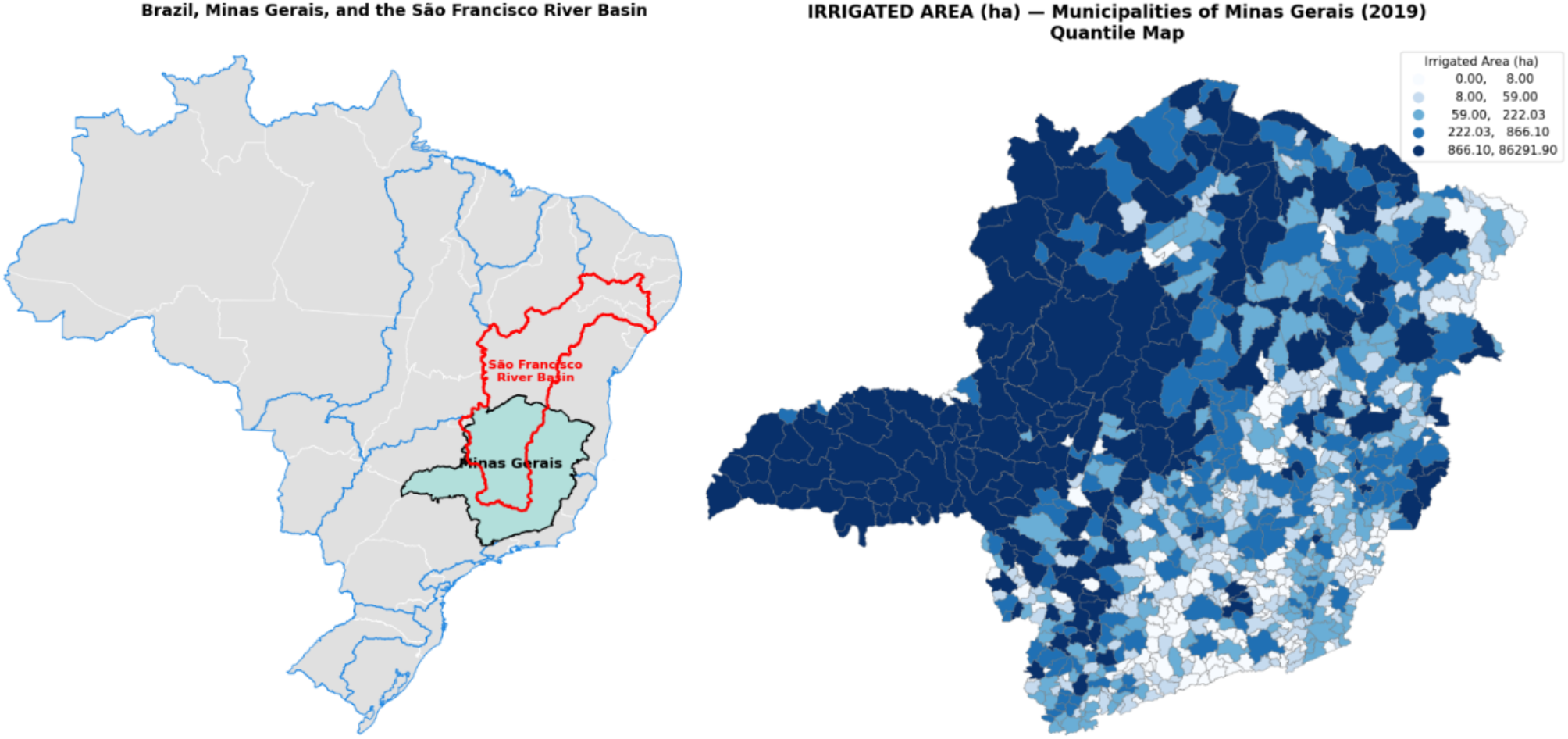
In 2019, water withdrawal in Brazil was distributed across livestock (8.4%), irrigation (49.8%), mining (1.7%), industry (9.7%), thermoelectric generation (4.5%), rural households (1.6%), and urban consumption (24.3%). Brazil’s irrigated area expanded from 4.5 million hectares in 2006 to 6.9 million hectares in 2017 and 8.2 million hectares in 2019. In Minas Gerais, the irrigated area increased from roughly 530,000 hectares in 2006 to about 1.12 million hectares in 2017 and 2019.
The Atlas of Irrigation (ANA, 2021) reports a national potential of 13.69 million hectares for additional irrigated agriculture, of which Minas Gerais accounts for approximately 8%, or nearly 1.14 million hectares. The state’s hydrological network comprises 17 federal river basins (Governo de Minas Gerais, 2020). Among them, the São Francisco river basin is the third-largest hydrographic basin in Brazil. Within Minas Gerais, it covers approximately 234,557 km2, encompassing 282 municipalities and serving an estimated 12.37 million inhabitants. Given this spatial heterogeneity and the inconsistencies in available data, a modelling strategy capable of distinguishing structural from informational zeros.
2.2. Database
The database employed in this study brings together information from the National Water and Basic Sanitation Agency (ANA) through the Irrigation Atlas (ANA, 2021), with a focus on irrigated area and potentially irrigable area in municipalities of Minas Gerais for the year 2019. Complementarily, data from the 2017 Agricultural Census, made available by the Brazilian Institute of Geography and Statistics (IBGE), were used to provide the rural numbers associated with cooperatives/associations per municipality.
For temporal consistency, it is assumed that data from the 2017 Agricultural Census remained constant in 20192. The selection of variables is guided by the literature highlighting the positive role of rural extension in improving productivity and rural development (Birkhaeuser et al., 1991; Da Silva, 2001). Municipal economic capacity, measured through agricultural gross value added (GVA), is included to capture the availability of economic resources. In addition, the inclusion of municipalities located within the São Francisco river basin reflects the expansion of irrigated areas in this region (Baiardi, Ribeiro, 2023).
To enhance data transparency and reproducibility, detailed data provenance is provided in Table 1, including the original data sources with specific table references. All variables were harmonised at the municipal level. Continuous covariates were standardised prior to estimation, and the dependent variable was log-transformed for positive observations. No missing values were identified in the original datasets, and the harmonisation process (including numeric conversion and standardisation) did not introduce additional missing observations3.
| Abbreviated name | General information | Source | Expected relationship | Variable type | Number of observations |
|---|---|---|---|---|---|
| area_irrig | Total irrigated area (hectares) per municipality | Irrigation Atlas – 2nd edition, online dataset (ANA, 2021) | Dependent variable | Continuous | 853 |
| assoc_coop | Number establishments with cooperatives/ associations per municipality |
Agricultural Census (IBGE, 2019), Table 6846 | Proxy for access to technology and markets; a positive relationship with irrigated area is expected | Continuous | 853 |
| receb_tec | Number of establishments receiving technical assistance per municipality | Agricultural Census (IBGE, 2019), Table 6779 | Proxy for human capital structure A positive relationship with irrigated area is expected |
Continuous | 853 |
| VAB_Agro | Gross agricultural value added (thousand R$), per municipality | IBGE (2021), Table 5938 | Proxy for municipal financial capacity | Continuous | 853 |
| Part_VAB | Share of agriculture in gross value added [GVA] (i.e., valor adicionado bruto [VAB]) per municipality |
IBGE (2021), Table 5938 | Proxy for the relative importance of agriculture in the local economy | Continuous | 853 |
| VAB_AD | Dummy: 1 if agricultural GVA < state average | IBGE (2021), Table 5938 | A positive relationship with structural zeros is expected | Binary | 1 = 647; 0 = 206 |
| Area_Pot | Dummy: 1 if the municipality has potential irrigable area | Irrigation Atlas (ANA, 2021), 2nd edition, online dataset | A negative relationship is expected, reducing the likelihood of a structural zero | Binary | 1 = 529; 0 = 324 |
| SF_Dummy | Dummy: 1 if located in the São Francisco river basin | Comitê da Bacia Hidrográfica do Rio São Francisco (CBHSF, 2025) (online dataset) | A positive relationship is expected, with a higher likelihood of irrigation | Binary | 1 = 239; 0 = 614 |
Each covariate is included based on its expected role in distinguishing structural from informational mechanisms. In the inflation component, SF_Dummy and Area_Pot capture geographical and hydrological feasibility, as municipalities located in the São Francisco river basin or with irrigable potential are less likely to face structural constraints to irrigation. The variable VAB_AD, defined as a dummy equal to 1 if agricultural GVA is below the state average, is used as a proxy for low economic capacity, associated with a higher likelihood of structural constraints to irrigation. In the continuous component, assoc_coop and receb_tec reflect access to information and technical support, respectively, which facilitate irrigation adoption conditional. Finally, VAB_Agro and Part_VAB capture the scale and economic relevance of agricultural activity, respectively, which are expected to be positively associated with irrigated area among municipalities with irrigation. Table 2 presents the descriptive statistics of the continuous variables employed in the model. High skewness and kurtosis indicate a concentration of low values alongside a few extreme observations, supporting the use of Student’s t-distribution.
| Statistics | area_irrig | assoc_coop | receb_tec | VAB_Agro | Part_VAB |
|---|---|---|---|---|---|
| Count | 853 | 853 | 853 | 853 | 853 |
| Mean | 1,341 | 293 | 186 | 30,952 | 13.42 |
| Standard deviation | 5,195 | 381 | 225 | 59,577 | 10.73 |
| Minimum | 0 | 0 | 1 | 44 | 0 |
| 25th percentile | 20 | 58 | 54 | 5,812 | 6.06 |
| 50th percentile | 114 | 165 | 114 | 12,241 | 10.76 |
| 75th percentile | 605 | 376 | 221 | 30,330 | 18.39 |
| Maximum | 86,291 | 2,910 | 2,131 | 782,041 | 62.24 |
| Skewness | 9.92 | 2.95 | 3.11 | 5.95 | 1.44 |
| Kurtosis | 130.18 | 11.91 | 13.63 | 51.14 | 2.54 |
2.3. Theoretical foundations of a zero-inflated model
Following Agarwal et al. (2002), the observed outcome is assumed to arise from a structural-zero component and a sampling distribution for positive observations. For a base distribution , the zero-inflated probabilities are:
(1)
(2)
where is the probability of excess zeros, and is the fraction following the base distribution. Covariates may influence both components of the model through separate linear predictors, typically via a log link for the continuous/count part and a logit link for the inflation probability.
(3)
(4)
where and are vectors of covariates for the count and zero-inflation components, respectively, and and are the corresponding parameter vectors. In other words, represents the expected outcome (e.g., irrigated area) conditional on being in the count process, while represents the probability of a structural zero. The next subsection presents the adaptation of this framework to irrigated agriculture in Minas Gerais.
2.4. A zero-inflated model for irrigated agriculture in Minas Gerais
Let denote the irrigated area (in hectares) for municipality i (I = 1, …, n), and assume that follows a zero-inflated model:
(5)
where denotes the probability of a structural zero. This specification corresponds to a two-part model, in which the zero outcome and the positive outcomes are modelled separately. The variable is defined only for municipalities with and is assumed to follow Student’s t-distribution with location , scale , and degrees . The exponential transformation ensures that predictions of irrigated area remain positive. Zero-inflation probability is linked to a set of covariates via a logistic regression:
(6)
where is a vector of covariates (including an intercept) and is the corresponding coefficients. For municipalities where irrigation is possible ( ), the expected log-irrigated area is modeled as:
(7)
where representing the standardised continuous covariates, and this component is estimated conditional on , implying a truncated likelihood for positive observations.
A Bayesian framework is adopted with weakly informative priors4. These priors are calibrated based on two considerations. First, the location parameters reflect the expected direction and approximate magnitude of effects, informed by descriptive statistics and preliminary regressions. In particular, the intercept is centred at a negative value to reflect the relatively low baseline probability of structural zeros. Second, Student’s t-distribution provides robustness to misspecification and allows for heavier tails compared with the normal distribution, and avoids sensitivity to extreme municipalities with unusually large, irrigated areas. Therefore, two specifications are simulated. Both models share the same structure defined above but differ in the set of covariates included in the inflation component. The inflation part in Model 1 (equation 8) is formally defined as:
(8)
where denotes the probability of a structural zero for municipality i, indicates whether the municipality belongs to the São Francisco river basin, indicates whether the municipality is below the average of the agricultural GVA (Agricultural), and denotes the presence of potential area for irrigation expansion. In Model 2 (equation 9), the inflation component includes an interaction term ( = × which captures the joint marginal effect of being located in the São Francisco river basin and having potential irrigable area ( ) defined as:
(9)
Model 2 extends Model 1 by including an interaction term between SF_Dummy and Area_pot, allowing the analysis to capture whether the effect of irrigable potential depends on geographical location within the São Francisco river basin. This specification is intended to test for heterogeneous effects in the probability of structural zeros, particularly in regions where water availability and irrigation infrastructure may condition the role of potential irrigable area. Predicted probabilities in the inflated component are obtained by transforming the linear predictor through the logistic function . Robustness is evaluated through 95% highest posterior density intervals (HDIs) and posterior probabilities of coefficient signs. Convergence is assessed using the statistic and visual inspection of trace plots, with Monte Carlo standard errors (mcse_mean and mcse_sd) and effective sample sizes (ess_bulk and ess_tail) reported for all parameters5.
To evaluate the influence of prior choices on posterior inference, a prior sensitivity analysis is conducted by re-estimating the Model 1 under an alternative set of less informative priors. In this specification, Student’s t priors originally assigned to the zero-inflation coefficients are replaced by diffuse normal6 priors centred at zero N(0,2), reducing the influence of prior location assumptions. For the continuous component, the coefficient priors are unchanged, while broader priors are adopted for the scale (σ ~ HalfNormal (1)), and ((ν ~ Gamma (2,0.5)) parameters. The model structure and data remain unchanged. In addition to the zero-inflated specification, a baseline model without zero inflation is estimated for comparison purposes. This model assumes that the logarithm of irrigated area follows a normal distribution for all observations, including those with zero values, which are adjusted by a small constant to enable the logarithmic transformation. It serves as a benchmark to assess whether the additional complexity of the zero-inflated model leads to improvements in predictive performance.
Predictive performance and model comparison
Predictive accuracy is evaluated using approximate leave-one-out cross-validation (LOO) and the widely applicable information criterion (WAIC), both computed from posterior samples (Vehtari et al., 2017). These criteria estimate the expected log predictive density (ELPD) and provide a measure of how well each model is expected to predict new observations. For the zero-inflated model, the predicted probability of structural zeros is directly obtained from the posterior distribution of . For the baseline model, which does not include a zero-generating mechanism, the predicted proportion of zeros is mechanically equal to zero. Comparing predicted and observed zero shares provides a direct test of whether the model captures the structural features of the data.
Finally, to examine heterogeneity in zero outcomes, the average predicted probability of structural zeros across different municipality types is computed, defined by key covariates such as location in the São Francisco river basin, irrigation potential, and agricultural GVA. This allows the assessment of whether zero outcomes are systematically associated with observable structural characteristics.
Spatial dependence assessment
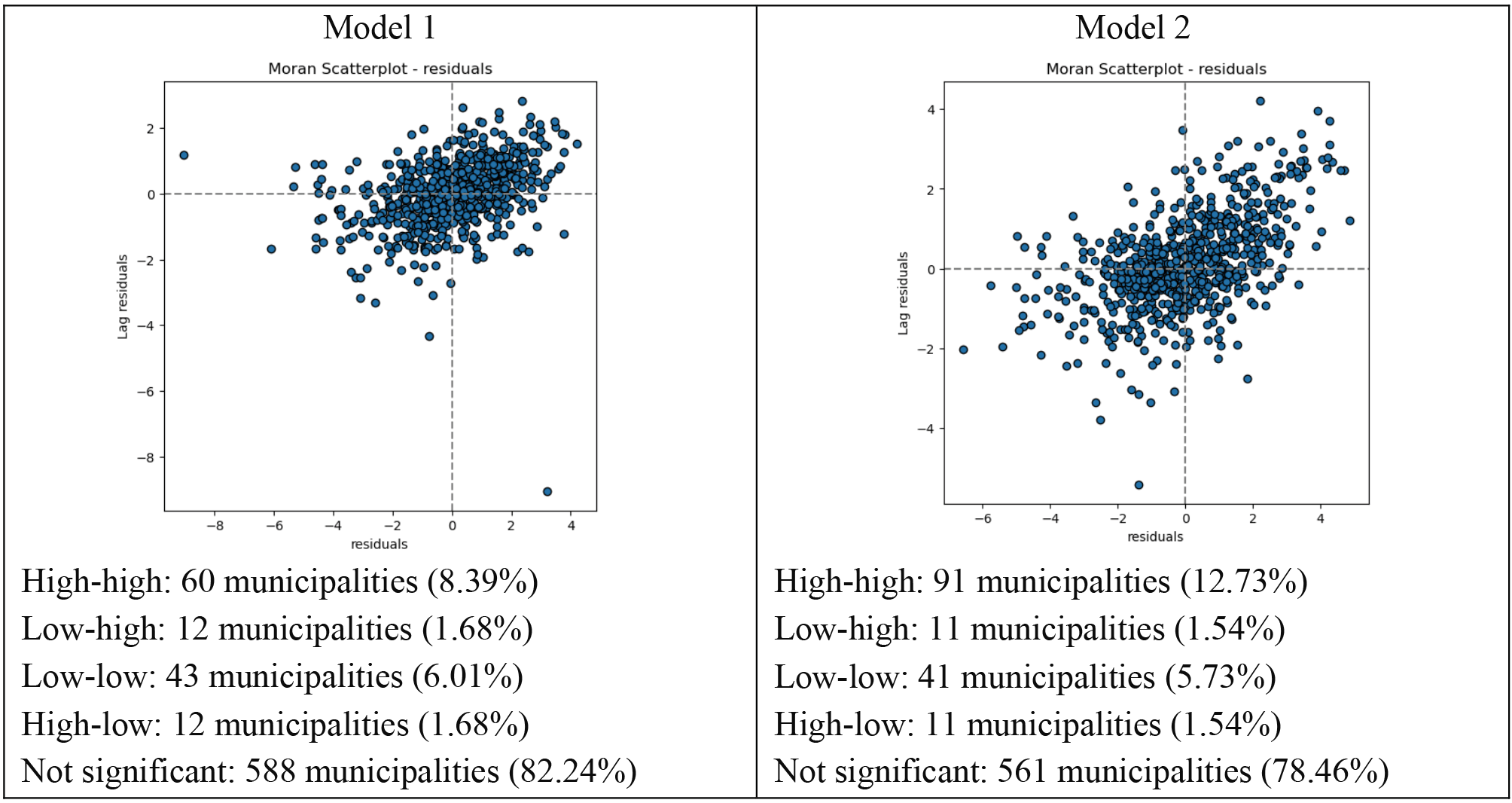
Although the models do not include explicit spatial random effects, residual spatial autocorrelation is assessed to determine whether the included covariates adequately capture spatial patterns. To this end, local Moran’s I (a local indicator of spatial association) on the residuals of the continuous component (Anselin, 1995) is used. Local Moran’s I for a standardised variable y, observed in region i, zi, can be expressed as (Almeida, 2012).
(10)
The calculation of considers only the neighbors of observation i, defined according to the spatial weight’s matrix , which in this study is specified using the queen contiguity criterion. Model estimation is performed via Markov chain Monte Carlo (MCMC) using PyMC v5.9.0 (2025), with posterior analyses conducted in ArviZ v0.16.1 for convergence diagnostics and exploratory assessment of the Bayesian results (Patil et al., 2010; Kumar et al., 2019). However, given that the residuals show no evidence of spatial autocorrelation, a parsimonious specification without spatial random effects is adopted.
3. Results
Due to the two-part structure of the zero-inflated model, the likelihood is evaluated using only positive observations in the continuous component. As a result, the number of effective observations differs across model components, preventing direct comparison using standard model ranking procedures. Therefore, LOO and WAIC are interpreted as within-model predictive diagnostics, rather than as strict model selection criteria across specifications (Table 3). The continuous component is estimated using only positive observations
(
), which implies a reduced effective sample size in that component of the likelihood. This feature is intrinsic to hurdle-type models and does not reflect missing data or sample selection.
| Model | elpd_loo | p_loo | WAIC | P_waic | Predicted zeros | Observations | |||||||||||||
|---|---|---|---|---|---|---|---|---|---|---|---|---|---|---|---|---|---|---|---|
| Log-normal | -2853.37 | 4.80 | -2853.32 | 4.75 | 0.00% | 853 | |||||||||||||
| Zero-inflated Student’s t | -1386.01 | 8.45 | -1385.97 | 8.41 | 21.67% | 715 | |||||||||||||
| Observed | — | — | 16.18% | ||||||||||||||||
| Note: The ELPD values are not directly comparable across the models due to different likelihood definitions and effective sample sizes. | |||||||||||||||||||
Table 3 indicates that the zero-inflated model improves predictive performance, particularly in capturing the presence of excess zeros, rather than merely providing a better in-sample fit. The sensitivity analysis indicates that the results depend on prior specification in the zero-inflation component. As discussed by Gelman (2006), priors intended to be noninformative or weakly informative can still exert a substantial influence on posterior inference. Under weakly informative priors, coefficients are well identified and consistent with theoretical expectations, and the model reproduces the observed zero share (≈20% vs 16.2%). In contrast, diffuse priors lead to weak identification, with coefficients shrinking toward zero (posterior mean ≈ 0.02) and wide credible intervals, substantially overestimating the proportion of structural zeros (≈50%). Furthermore, the zero-inflated model reveals substantial heterogeneity in predicted zero probabilities across municipality types. Predicted zero probabilities are higher outside the semi-arid region (26.1% vs 10.3%), in municipalities without irrigation potential (35.1% vs. 13.5%), and among those with lower agricultural value added (26.7% vs. 5.9%).
Convergence diagnostics indicate stable MCMC performance across all specifications, with low Monte Carlo standard errors (≈0.001) and satisfactory mixing in both the central and tail regions of the posterior distributions. The inflation component models the probability of structural zeros via a logit specification, while the continuous component captures the magnitude of irrigated area conditional on positive observations. The parameter estimates for Model 1 and Model 2 are reported in Tables 4 and 5, respectively.
| Component | Variable | Mean | 3% hdi | 97%hdi | MCSE mean |
MCSE sd |
ESS bulk |
ESS tail |
|
|---|---|---|---|---|---|---|---|---|---|
| Inflated part | Intercept | -2.00 | -3.47 | -0.56 | 0.013 | 0.012 | 6365 | 3304 | 1 |
| SF_Dummy | -0.99 | -1.88 | -0.17 | 0.006 | 0.007 | 8246 | 3521 | 1 | |
| VAB_AD | 1.48 | 0.61 | 2.37 | 0.007 | 0.005 | 7792 | 3233 | 1 | |
| Area_pot | -1.00 | -1.82 | -0.20 | 0.005 | 0.005 | 9275 | 3802 | 1 | |
| Intercept | 5.28 | 5.15 | 5.39 | 0.001 | 0 | 8897 | 6202 | 1 | |
| Count part | assoc_coop | 0.28 | 0.16 | 0.39 | 0.001 | 0 | 7605 | 6361 | 1 |
| VAB_Agro | 1.07 | 0.89 | 1.25 | 0.001 | 0.001 | 6063 | 6088 | 1 | |
| receb_tec | 0.12 | -0.01 | 0.25 | 0.001 | 0.001 | 6384 | 6079 | 1 | |
| Sigma (σ) | 1.46 | 1.33 | 1.58 | 0.001 | 0.001 | 5065 | 5359 | 1 | |
| Nu (v) | 10.38 | 4.56 | 18.73 | 0.079 | 0.056 | 4609 | 4069 | 1 |
| Component | Variable | Mean | 3% hdi | 97%hdi | MCSE Mean |
MCSE sd |
ESS bulk |
ESS tail |
|
|---|---|---|---|---|---|---|---|---|---|
| Inflated Part | Intercept | -1.97 | -3.39 | -0.468 | 0.009 | 0.008 | 8469 | 3454 | 1 |
| SF_Dummy | -1.00 | -1.82 | -0.119 | 0.006 | 0.006 | 8805 | 3681 | 1 | |
| VAB_AD | 1.48 | 0.63 | 2.374 | 0.007 | 0.005 | 7538 | 3547 | 1 | |
| Area_pot | -0.98 | -1.84 | -0.063 | 0.007 | 0.008 | 7846 | 2751 | 1 | |
| SF_interação | -0.50 | -1.93 | 0.865 | 0.012 | 0.018 | 7146 | 3234 | 1 | |
| Count Part | Intercept | 5.26 | 5.14 | 5.385 | 0.001 | 0.001 | 8503 | 5829 | 1 |
| assoc_coop | 0.39 | 0.26 | 0.516 | 0.001 | 0.001 | 7562 | 6038 | 1 | |
| Part_VAB | 0.51 | 0.39 | 0.639 | 0.001 | 0 | 9162 | 6305 | 1 | |
| receb_tec | 0.51 | 0.38 | 0.657 | 0.001 | 0.001 | 7510 | 5997 | 1 | |
|
Sigma ( |
1.64 | 1.52 | 1.759 | 0.001 | 0.001 | 6458 | 6583 | 1 | |
| Nu (v) | 16.00 | 5.76 | 30.918 | 0.112 | 0.081 | 6200 | 5530 | 1 |
The intercepts provide the baseline reference for each model component. In the inflated part, the intercept of -2.007 corresponds to a baseline probability of 11.9% that a municipality is a structural zero when all predictors are held at their mean values. In the continuous part, the intercept of 5.28 indicates an expected irrigated area of approximately 196.4 hectares, given that irrigation is present.
For the inflated component, the results are presented as predicted probabilities to enhance interpretability. Belonging to the São Francisco river basin (SF_Dummy = 1) reduces the probability of a structural zero from 11.9% to approximately 4.7%7, indicating that municipalities in this basin are less likely to lack irrigation. In contrast, municipalities with agricultural GVA below the state average (VAB_AD = 1) have a higher probability of being structural zeros, increasing from 11.9% to about 37.4%. The presence of irrigable area (Area_pot = 1) also decreases the structural-zero probability to around 4.7%, reinforcing the importance of land suitability in reducing the likelihood of zero irrigation.
In the continuous component, covariates are standardised (mean = 0, standard deviation = 1), and the results are expressed as percentages to improve comparability across the variables. The variable assoc_coop (0.289) implies that a one-standard-deviation increase in the proportion of farmers associated with cooperatives is associated with an approximate 33%8 increase in the log-mean irrigated area, highlighting the positive role of corporativism. The coefficient for VAB_Agro (1.073) corresponds to an increase of about 192% in the expected irrigated area, revealing a strong association between agricultural GVA concentration and irrigation intensity. Finally, receb_tec shows a positive but more uncertain effect: the estimated coefficient (0.121) implies a 12.9% increase, but the posterior interval includes zero, indicating limited statistical certainty about this relationship.
Model 2 (Table 5) introduces an interaction term (SF_interação), identifying 194 municipalities that simultaneously belong to the São Francisco river basin and possess irrigable potential. The interaction coefficient indicates that when both conditions are jointly satisfied (São Francisco river basin and irrigable potential), the interaction term reduces the probability even further, to approximately 1.1% (-0.509), indicating a strong combined protective effect against the absence of irrigation. However, the HDI includes zero, indicating uncertainty in the effect direction in the inflation component.
In the continuous component of Model 2, the results remain consistent with those of Model 1. The presence of more associations and cooperatives is positively associated with larger irrigated areas, and municipalities receiving greater technical support also exhibit a higher irrigated area. The relative participation variable in agricultural GVA shows a positive and statistically significant effect, although smaller than the absolute GVA measure used in Model 1, likely reflecting its lower variability (see Table 1). Additionally, in Model 2, the variable receb_tec becomes statistically significant, indicating improved overall model. The increase in v = 16 in Model 2 suggests that the interaction term captured part of the extreme variability, resulting in lighter tails compared to Model 1. Table 6 provides a summary of the predicted structural-zero probabilities for both models.
| Model 1 | Model 2 | ||||
|---|---|---|---|---|---|
| Variables | Logit (n) | Predicted probability | Variables | Logit (n) | Predicted probability |
| Baseline | -2.007 | 11.9% | Baseline | -1.972 | 12.2% |
| SF_Dummy | -0.996 | 4.7% | SF_Dummy | -2.978 | 4.8% |
| VAB_AD | 1.489 | 37.4% | VAB_AD | 1.486 | 38.1% |
| Area_pot | -1.005 | 4.7% | Area_pot | -2.959 | 4.9% |
| SF_interação | -4.474 | 1.1% | |||
The baseline probability of a structural zero remains around 12%, but this probability drops to approximately 5% in municipalities located in the São Francisco river basin or those with potential irrigable area. In contrast, municipalities with agricultural GVA below the state average exhibit higher probabilities of structural zeros (around 38). In Model 2, the interaction term indicates that municipalities simultaneously located in the São Francisco river basin and endowed with potential irrigable area have the lowest probability of structural zeros (about 1%), suggesting a strong combined mitigating effect.
Figure 2 presents the posterior distributions of the mean probability of structural zeros ( across municipalities in Minas Gerais to assess the predicted effects on structural zeros from Models 1 and 2. The distributions show that both models estimate a higher proportion of structural zeros than observed. Some considerations follow: (i) according to the 2017 Agricultural Census, which collected data directly from farmers, only 6% of municipalities reported no irrigation; (ii) Irrigation Atlas estimates are indirect, based on remote sensing, hydrological models, imputations, and other data sources, resulting in 16.8% zeros.
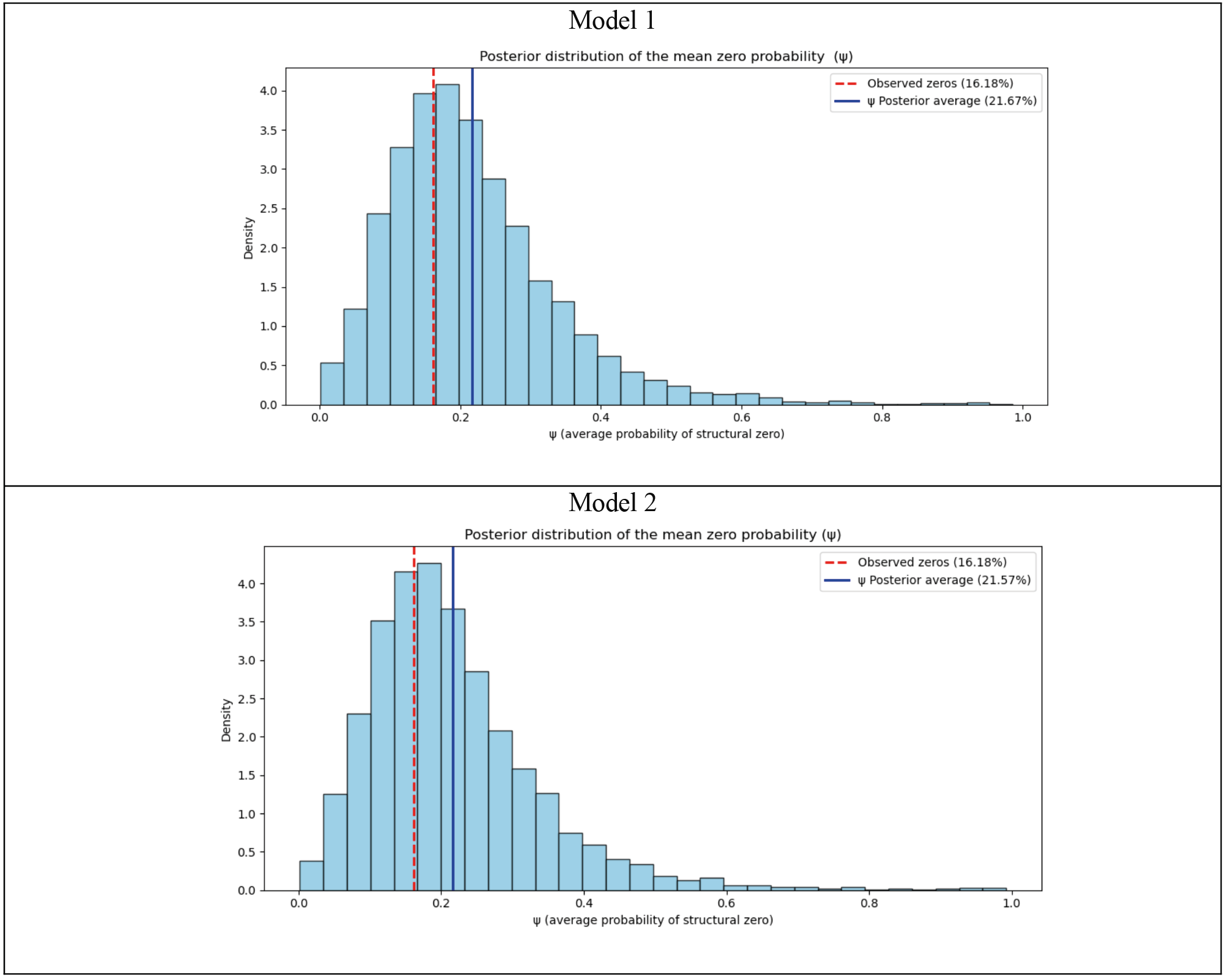
Figure 2. Posterior distribution of the mean zero probability .