Research article
Environmental vulnerability in Italian mountain areas and its socioeconomic drivers
1 Department of Economics, Statistics and Business, Universitas Mercatorum, Italy
2 Department of Biosciences and Territory, University of Molise, Campobasso, Italy
3 Department of Economics, University of Molise, Pesche (IS), Italy
*Corresponding author. E-mail: a.cavallo@unimercatorum.it
Abstract. Mountain areas are exposed to multiple risks due to the complex interactions between environmental, social, and economic factors. This paper aims to assess the environmental vulnerability of mountain areas through a synthetic indicator and to identify the drivers of such vulnerability at the local level. It uses a multidimensional and spatial approach to define the main dimensions of vulnerability based on municipal data. Furthermore, a geographically weighted regression model is used to investigate the drivers of vulnerability. The results show that mountain areas are less environmentally fragile than lowland and hilly regions but have higher demographic, social, and economic vulnerability. However, southern mountains are more fragile due to the lower presence of protected areas and forest cover. The spatial model also reveals a trade-off between environmental preservation and demographic, social, and economic characteristics. These findings should be carefully considered in light of place-based planning strategies and policies in mountain areas, particularly in southern Italy.
Keywords: vulnerability, composite indicators, spatial analysis, GWR model, planning.
JEL codes: Q15, Q18, R58.
Index
2.1. Dataset and variables definition
2.2. Derivation of the synthetic indexes
2.3. The spatial econometric model
Highlights
– Mountain areas are prone to multiple environmental hazard factors
– A vulnerability index to analyse the environmental state of Italian mountain is defined
– Several socio-economic drivers are investigated at the spatial scale
– Mountain areas show a healthier environmental condition than hill and plain zones, with a trade-off between environment and socio-economic features
– The research findings provide useful insights for planning strategies
1. Introduction
Research on human-environment vulnerability primarily considers large-scale environmental processes (Cutter et al., 2014; UNDRO, 1979) and identifies various areas of vulnerability, including economic, social, and environmental factors, as well as the complex relationships linking these factors to risk (Cutter, 2021). The spatial variation of vulnerability and the factors that cause it is pivotal to the development of policy measures aimed at strengthening the resilience of the most exposed communities (UNISDR, 2015). Vulnerability can be conceptualised as the consequence of multiple spatial marginalities that are interdependent in their dynamic evolution (Vendemmia et al., 2021). This approach facilitates the identification of differential degrees of spatial marginality, which is instrumental in the recognition of varied intensities and manifestations of vulnerability, thus enabling the formulation of targeted spatial policies (OECD, 2022). While this issue has been investigated more extensively in urban areas (Sun et al., 2022), vulnerability analysis remains a crucial aspect in marginal areas, particularly mountain areas, which are more exposed to environmental risks (Karpouzoglou et al., 2020).
Vulnerability is a multidimensional concept (Bernués et al., 2022; Ford et al., 2018) linked to a population’s exposure to hazards and its ability to respond to and recover from the impacts of such risks (Thorn et al., 2020). Mountain communities have different capacities for resilience and recovery depending on their social and economic conditions (Jha et al., 2021). Therefore, in mountain areas, the incidence of multi-risk events and the causal links between risks are often deeply intertwined (Schmeller et al., 2022). For example, earthquakes can trigger secondary processes such as avalanches or landslides, and droughts are deeply linked to fires. Multi-hazard risks pose a major challenge because they are expected to increase in intensity and frequency with global warming (Bankoff, Hilhorst, 2022). These risk categories need to be analysed separately because manageable threats can be addressed, while unavoidable ones can only be mitigated and are generally associated with environmental risks (Mastronardi et al., 2022).
Multiple pressures have affected mountain areas in recent decades, including demographic decline and depopulation (González-Leonardo et al., 2022), abandonment of agricultural activities (Levers et al., 2018), and the dependence of local economies on tourism (Teare, 2021). Since the 1950s, Italian mountains have experienced a demographic decline and population ageing, leading to an uneven socio-economic fabric and a severe lack of essential services. These conditions favour a vicious circle which accelerates population abandonment, reduces economic activities, and leads to the disintegration of the social fabric and the increase in land management costs (Pagliacci, Russo, 2019).
Italian mountain areas have multiple vulnerabilities. The impact of earthquakes is often devastating, and the fragile socio-economic structure of these places emerges as a critical factor in earthquakes, particularly in the Apennine areas (Pagliacci et al., 2021). Landslides have a significant impact in terms of loss of life and natural resources (Trigila, Iadanza, 2018), which can be exacerbated by the impact of climate change in inner areas, both in terms of frequency (Gariano et al., 2018) and intensity (Esposito et al., 2023). These events are also linked to the abandonment of agriculture, which has accelerated in mountain areas (Dax et al., 2021), leading to changes in land use and forest cover (Rumpf et al., 2022). These changes have been confirmed by future change models (Gobiet, Kotlarski, 2020).
Italian mountain areas have the highest percentage of forests and protected areas in the country, along with lower levels of air pollution and land consumption (Uncem, 2025). Forests provide ecosystem services and socio-economic benefits (Dasgupta, 2021), and contribute to climate change mitigation (Callisto et al., 2019). Protected areas play a crucial role in biodiversity conservation and sustainable development (Acreman et al., 2020). Mountains are socio-ecological systems whose management and conservation are linked to human activity (Bretagnolle et al., 2019). As such, they have a positive impact on the provision of ecosystem services (Kokkoris et al., 2018), income (Sena-Vittini et al., 2023), and employment (Acampora et al., 2023) through the enhancement of tourism (Lenart-Boroń et al., 2021), and sustainable, quality-conscious agricultural practices (Romano et al., 2021).
The relationship between socio-economic factors and environmental conditions is crucial in mountain areas. The weakness of socio-economic factors, such as depopulation, ageing, a decline in employment, and the cessation of business activities, impacts the abandonment of territory (Urso et al., 2019). Consequently, these areas are subjected to environmental vulnerability (i.e., landslides and hydrogeological instability), thereby increasing remoteness (Di Giovanni, 2016; Pilone, De Michela, 2018). Many economic and social indicators can contribute to the measurement of vulnerability, but there are still research gaps regarding the identification of indicators that allow for the measurement of when a population or area is exposed to multiple environmental risks (Cong et al., 2023). This requires the need of appropriate spatial scales, including the local ones, to effectively address risk management and the concerns of stakeholders and local communities (Marsden, 2024).
The aims of the study are (1) to assess the environmental vulnerability of mountain areas through the definition of a synthetic indicator; and (2) to identify the drivers of such vulnerability at local level. This study addresses some gaps in the literature by using a multidimensional and spatial approach that has been less explored in the literature (Drakes, Tate, 2022; Schmeller et al., 2022), especially in mountain areas, which are more exposed to multiple risk and threat factors (Eckstein et al., 2021). The distinctive contribution of this research lies in the integration of environmental and socio-economic vulnerability at a spatial level, a critical aspect of human-environment interactions, into the assessment of mountain exposure to environmental risks (Pirasteh et al., 2024).
The remainder of this paper is organised as follows. Section 2 describes the data and methods used for our analysis. Sections 3 and 4 present the results and discuss them. Finally, Section 5 provides the conclusions.
2. Dataset and methods
2.1. Dataset and variables definition
To construct a composite vulnerability index, we analysed the available datasets on the selected variables for the Italian municipalities. On 1 January 2019, Italy was subdivided into 7960 municipalities; our data refer to 7942 of them, due to missing data for the remaining 18. Our interest is in mountain areas, comprising 2514 municipalities classified as “Inner Mountain” (2397) or “Coastal Mountain” (117) by the Italian National Institute of Statistics (Istat).
The variables and indicators considered are reported in Table 1. Apart from previous considerations described in Section 1, the selection of variables integrates environmental and socio-economic aspects to ensure a comprehensive assessment of the multiple factors that shape vulnerability when using a spatial approach. Nevertheless, the choice of variables was heavily conditioned by the information available at the municipal level. We used the most recently data available for 2017-2019, with the exception of data pertaining to the 2020 so-called National Strategy for Inner Areas (IANS). When necessary, we normalised the original variables to eliminate the scale effects deriving from the very different size of the municipalities.
| Variable | Source* | Indicator | Acronym | Domain** | |||||||||||||||
|---|---|---|---|---|---|---|---|---|---|---|---|---|---|---|---|---|---|---|---|
| Earthquake hazard | INGV | Earthquake hazard classification | EH | Environment | |||||||||||||||
| Landslide hazard | ISPRA | Share of landslide hazard areas | LH | Environment | |||||||||||||||
| Flood hazard | ISPRA | Share of flood hazard areas | FH | Environment | |||||||||||||||
| Monthly average precipitation | CRU-UEA | Abnormal Standardised Precipitation Index | A_SPI | Environment | |||||||||||||||
| Particulate matter pollution | ISPRA | Particulate matter pollution | PM10 | Environment | |||||||||||||||
| Waste collection | ISPRA | Per capita waste collection | WA | Environment | |||||||||||||||
| Land consumption | ISPRA | Share of land consumption | LC | Environment | |||||||||||||||
| Forest areas | CLC | Share of forest areas | FA | Environment | |||||||||||||||
| Protected areas | UN-WCMC | Share of protected areas | PA | Environment | |||||||||||||||
| Population aged 80+ | Istat | Share of population aged 80+ | EP | Demography | |||||||||||||||
| Births and deaths | Istat | Natural growth rate | NGR | Demography | |||||||||||||||
| Degree of urbanisation | Istat | (Modified) Population density | MPD | Society | |||||||||||||||
| IANS | Istat | Time of travel to the nearest Pole | TNP | Society | |||||||||||||||
| Local units | Istat | Local units per 1000 residents | UL | Economy | |||||||||||||||
| Employees | Istat | Employees per 1000 residents | EMP | Economy | |||||||||||||||
| Note: *INGV, Italian Institute of Geophysics and Volcanology; ISPRA, Italian Institute for Environmental Protection and Research; CRU-UEA, Climatic Research Unit – University of East Anglia; CLC, Corine Land Cover; UN-WCMC, UN Environment Programme – World Conservation Monitoring Centre; Istat, Italian National Institute of Statistics. | |||||||||||||||||||
| ** Each background colour refers to a different synthetic index (described in Section 2.2). Green: SEVI; light orange: DWI; orange: SDI; light blue: EWI. | |||||||||||||||||||
We considered the impact of variables on the environmental, demographic, social and economic domains to justify their inclusion. The effects and related literature are reported in Table 2.
The methodological approach consists of two phases, related to the two goals stated at the end of Section 1. They are described in the following subsections.
| Variable | Effects | Reference literature |
|---|---|---|
| Earthquake hazard | Damage to buildings, Infrastructure, and people | European Commission, 2021 |
| Landslide hazard / flood hazard | Modify the natural environment and hit communities as a whole | Aroca et al., 2022; Trigila, Iadanza, 2018 |
| Monthly average precipitation | Too much rain triggers floods and landslides Long-term dryness: soil erosion, salinisation, and land degradation |
European Environment Agency, 2020 |
| Particulate matter pollution | Danger to human health, especially in urban areas | Brooks, Sethi, 1997 |
| Waste collection | Negative effects on air, soil, and water pollution | ISPRA, 2020 |
| Land consumption | Non-reversible soil use or transformation | ISPRA, 2018 |
| Forest areas | Carbon dioxide capture, release of water vapour, conservation of plant and animal life and reduction of hydrogeological risk | IPCC, 2023 |
| Protected areas | Biodiversity and ecosystem conservation | Geldmann et al., 2013; Stolton et al., 2015 |
| Population aged 80+ years | Low dynamism and less available workforce | Mottet et al., 2006 |
| Births and deaths | Demographic decline, abandonment of productive activities, and loss of social capital |
Jha et al., 2021; Pilone, De Michela, 2018 |
| Degree of urbanisation | Rurality condition and economic disadvantage | De Rossi, 2018 |
| Distance from the nearest Pole | Remoteness from essential public services | Uval, 2014 |
| Local units | Resilience and vitality of the productive fabric | Urso et al., 2019 |
| Employees | Vitality of social capital | Faggian et al., 2018 |
2.2. Derivation of the synthetic indexes
The first phase involved nine variables related to the environmental domain (Table 1). We maintained the original value (level of risk) of the indicators earthquake hazard (EH) and particulate matter pollution (PM10) and considered them quantitative variables. We derived landslide hazard (LH), flood hazard (FH), land consumption (LC), protected areas (PA), and forest areas (FA) by dividing the original values by the corresponding municipal areas. Waste collection (WA) is the annual waste per inhabitant (in kilograms). Finally, we calculated monthly average precipitation (A_SPI; the Abnormal Standardised Precipitation Index) as follows. The standardised precipitation index (SPI) was determined as SPI-12 (12 months of accumulation) (Bordi et al., 2007) over a 30-year period and after the time series (one for each municipality). Then, we calculated the fraction of times for which |SPI| > 1.5: , giving the same consideration to drier and wetter periods when defining its contribution to vulnerability.
We used the aforementioned indicators to build the synthetic environmental vulnerability index (SEVI). Seven of the indicators have a direct relationship to SEVI; this means that an increase of an indicator leads to an increase in SEVI, and vice versa. FA and PA, however, are inversely linked to environmental vulnerability. Therefore, we modified their original values, denoted by FAi and PAi, to become FAinv,i = 1 – FAi and PAinv,i = 1 – PAi, which range from 0 (no vulnerability, when the whole municipal territory is covered by forests and/or protected areas) to 1 (maximum vulnerability, in the absence of forests and/or protected areas). We also standardised all indicators to give each the same weight. The resulting index is defined for the i-th municipality (i = 1,…,7942) as the mean , where ZIj is the j-th standardised indicator. By definition, SEVI has a mean of 0 and variance that is less than 1 (because it is a linear combination of correlated standardised variables).
For the second phase, we built three more synthetic measures that can be considered proxies for the demographic, social, and economic features of Italian municipalities. We used them to analyse the relationships among environmental vulnerability, as expressed through the SEFI measure, and the socio-economic fabric at a local scale.
The demographic weakness index (DWI) includes the share of population aged 80+ years and the natural growth rate. The latter is defined as the difference between the number of births and deaths in a given year, divided by the average amount of the resident population and multiplied by 1000.
The social disadvantage index (SDI) is defined as vulnerability caused by the scarcity of so-called essential services (health, education, and mobility services). Thus, this index can be based on the degree of urbanisation and the IANS classification, as both reflect social distress due to a lack of services. The degree of urbanisation is expressed through transformation of the population density (PD). Because PD is hypothesised to be inversely linked to the presence of essential services, we first calculated the square root of PD to reduce the variability and then took the inverse of that result. Consequently, the modified population density employed is . With regard to the IANS classification, the indicator employed is the time of travel (by public transport), in minutes, to reach the nearest Pole (in the context of the IANS, a Pole indicates a municipality where all the essential services are present).
Finally, the economic weakness index (EWI) includes the number of local units of firms per 1000 residents and the number of employees per 1000 residents.
Just like for SEVI, we calculated DWI, SDI, and EWI by standardising each component. We employed the mean values of each index as independent variables in the local spatial model.
2.3. The spatial econometric model
As discussed in Section 1, the social, institutional, and economic characteristics of local communities directly influence the evolution of ecosystems and environmental condition (Carrer et al., 2020; Jha et al., 2021; Stotten et al., 2021; Whitaker, 2023). To model this relationship, we used a geographically weighted regression (GWR) model (Fotheringham et al., 2002). Given a set of multivariate observations, geographically set in n sites (or zones or locations), on P independent variables and one dependent variable, GWR belongs to the class of spatially varying coefficient (SVC) models. They consider spatial heterogeneity in the coefficients and are employed especially when large samples are available (Murakami et al., 2020). Most of the approaches to SVC problems, however, are affected by the ‘degeneracy problem’: they use spatially varying local functions that are too smooth and produce map representations of the coefficients that fail to capture local-scale coefficient variations. Thus, GWR is a very useful tool because it is not affected by degeneracy. It allows for more realistic modelling of local characteristics based on the choice of several local kernels.
Formally, GWR is a non-parametric model based on a sequence of locally linear regressions, built to produce estimates for every point in space using a sub-sample of data information from nearby observations (LeSage, 2004). The GWR model gives rise to distinct local regressions, one for each site. Drawing on Tobler’s first law of geography (Tobler, 1970), which states that nearby phenomena tend to occur in a more similar way than distant ones, we adopted this local spatial model because estimating a single parametric value for the entire observed area – as in conventional (non-spatial) regression – would be impractical.
The observations in each of the distinct equations are based on a set of local weights. Hence, each observation has importance that decays as distance from site i under consideration increases. The -th local GWR can be expressed, in matrix-vector form, as:
(1)
where is the n × 1 vector of the dependent variable; is the n × (P + 1) matrix of the independent variables, with , the n × 1 vector of ones, in order to include in the equation, the intercept term ; is the , a dimensional vector of the -th local model parameters; , , …, is an n × n diagonal matrix that, in the j-th position of the main diagonal, contains the distance-based weight measuring the distance between observations at sites i and j; and is the error term relating to i-th local regression: .
The (local) parameter estimates for the model in Equation (1) are obtained through weighted least-squares and written as:
(2)
where, as usual, indicates the transpose of . The result in Equation (2) depends on a bandwidth, b, which characterises the chosen local kernel function and determines the weights to be assigned to the neighbouring observations of site i. The usual choice for the weights exploits Euclidean distance and a Gaussian distance-decaying kernel (Lu et al., 2022):
(3)
with dij representing the Euclidean distance between zones i and j. The choice of an optimal value for the bandwidth is a crucial point for any GWR. The task is typically solved by means of a leave-one-out cross-validation (LOOCV) procedure to minimising the cross-validation score, CV: , where is the fitted value for yi which derives from an estimation procedure leaving out the i-th observation.
The LOOCV step is computationally very demanding, as are also the calculations required by the diagnostics, commonly based on an adjusted R2 ( ) and/or a corrected Akaike information criterion (AICc). These steps involve a high number of repeated calculations on large matrices, which often makes the use of a GWR unfeasible in the presence of big databases. For these reasons, many possible alternatives to ‘classical’ GWR have been proposed in the scientific literature (for a review and comparison among different methods, see Lu et al., 2022).
To analyse our data, we chose to employ the scalable GWR model (ScaGWR) proposed by Murakami et al. (2020). This method replaces the standard non-linear kernels present in GWR analysis with a linear multiscale kernel of the form:
(4)
where
is a base kernel, assumed to be a decreasing function of distance dij and have a value of 1 for dij} = 0; b* is a fixed bandwidth; K is the maximum order of the polynomials defining the multiscale kernel; and Q is the number of neighbours of site i, a fixed number for every local kernel of the type in Equation (4). It is used to determine the threshold for the base kernel. Letting
be the distance between site
and its Q -th nearest neighbour, it will be
if
,
and
. Having fixed b*, K, and Q, the estimated parameters are
, a global weight parameter, and
,which weights the local terms of Equation (4).
There are two especially relevant advantages of the ScaGWR model. First, it drastically reduces the computational burden to find parameter estimates. Specifically, are defined at a cost of complexity O(nQ) instead of O(N2), and the LOOCV procedure for estimating ɑ and γ has a cost, which is quasi-linear with respect to n. Second, ad hoc simulations have highlighted that the local parametric estimates obtained through ScaGWR are at least as good, in terms of the root mean square error (RMSE), as those obtained through classical GWR. This means that they can be usefully employed in cases like ours: with an n close to 8000, there can be problems in running a standard GWR algorithm.
3. Results
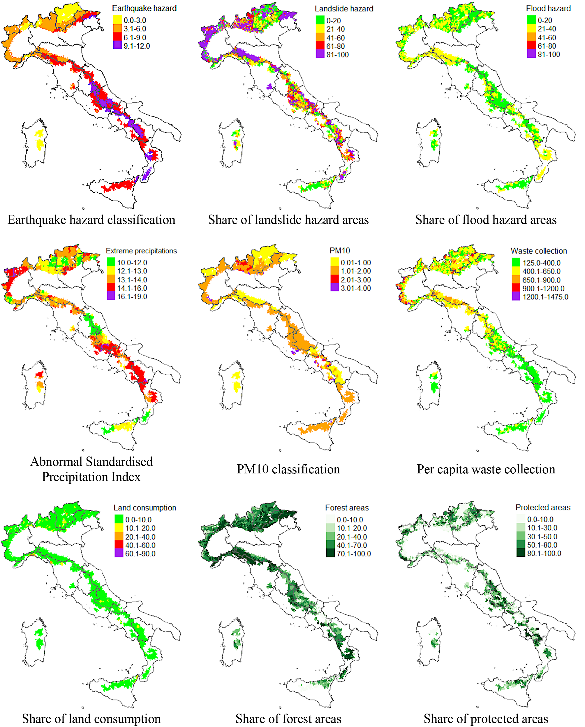
Table 3 reports the mean values of the environmental indicators introduced in Table 1. Mountain areas show the highest values for EH, LH, FA, and PA. However, they show the lowest values for PM10 and LC, indicators that are related to a better environmental condition. The remaining indicators for the mountain areas are near or equal to the national mean. Maps showing the geographical distribution of the original indicators in Mountain Areas (MAs) are reported in Figure A.1 in the Appendix.
| Altimetric zone | EH | LH | FH | A_SPI | PM10 | WA | LC | FA | PA | ||||||||||
|---|---|---|---|---|---|---|---|---|---|---|---|---|---|---|---|---|---|---|---|
| Plain | 5.50 | 0.09 | 0.14 | 0.13 | 3.60 | 476.43 | 0.17 | 0.05 | 0.06 | ||||||||||
| Hill | 6.96 | 0.47 | 0.16 | 0.14 | 2.19 | 427.25 | 0.10 | 0.25 | 0.14 | ||||||||||
| Mountain | 7.19 | 0.54 | 0.15 | 0.13 | 1.64 | 455.01 | 0.04 | 0.61 | 0.27 | ||||||||||
| Italy | 6.64 | 0.39 | 0.15 | 0.14 | 2.39 | 449.02 | 0.10 | 0.31 | 0.16 | ||||||||||
| Note: EH is based on four-class classification (low, medium, high, very high). LH is the share of landslide hazard municipal areas. FH is the share of flood hazard municipal areas. A_SPI is the fraction of times (over a 30-year period) for which the Standardised Precipitation Index exceeds the value of 1.5. PM_10 is presented as µg/m³. WA is presented as kilograms per capita. LC is the share of municipal land consumption. FA is the share of forest municipal areas. PA is the share of protected municipal areas. | |||||||||||||||||||
Table 4 shows the SEVI median, mean, and standard deviation (SD) for each altimetric zone and for Italy as a whole. SEVI decreases gradually when moving from plain to hill to mountain areas. Within the individual zones, the variability is quite high, as indicated by the SDs.
| Altimetric zone | Median | Mean | SD |
|---|---|---|---|
| Plain | 0.178 | 0.193 | 0.274 |
| Hill | 0.067 | 0.043 | 0.336 |
| Mountain | -0.212 | -0.220 | 0.330 |
| Italy | 0.022 | 0.000 | 0.357 |
At the municipal level, Figure 1 illustrates the SEVI values for mountain areas. There are some critical situations in north-western Italy, and some in the central and southern parts of the country.
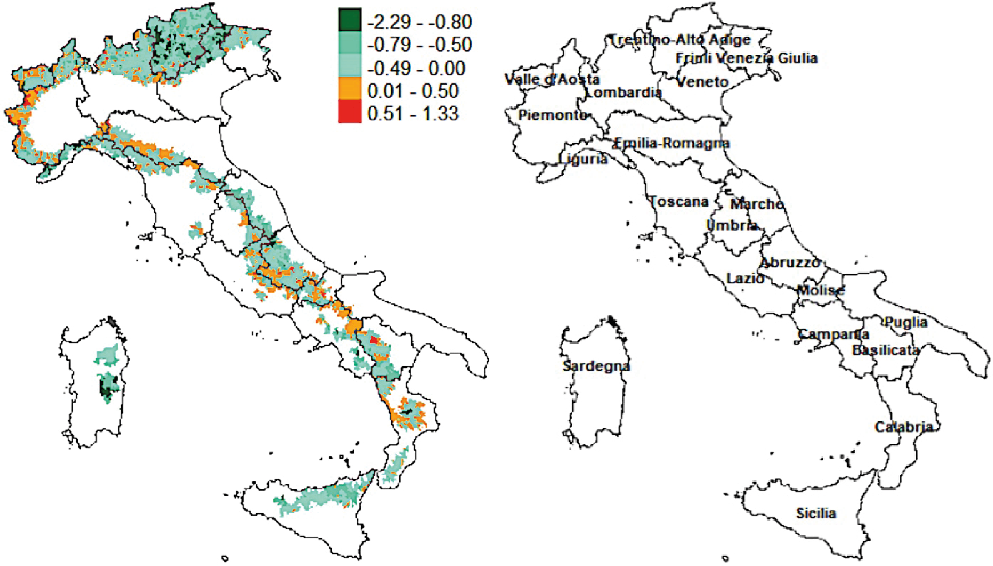
Table 5 provides details for the municipalities with a SEVI > 0 (i.e., the most fragile ones). There is still an apparent decrease in terms of the percentage of municipalities involved and their surface area when going from plain to mountain areas. The population living in fragile areas is higher in hill municipalities in both absolute and relative terms.
| Altimetric zone | Number of municipalities |
Surface area (km2) |
Population | ||||||||||||||||
|---|---|---|---|---|---|---|---|---|---|---|---|---|---|---|---|---|---|---|---|
| Plain | 1650 (78.31) |
32,666.95 (46.75) |
9,909,398 (33.49) |
||||||||||||||||
| Hill | 1912 (57.57) |
41,763.60 (33.34) |
11,150,821 (47.58) |
||||||||||||||||
| Mountain | 642 (25.54) |
11,916.28 (11.21) |
2,925,309 (39.60) |
||||||||||||||||
| Italy | 4204 (52.93) |
83,346.83 (28.64) |
23,985,528 (39.70) |
||||||||||||||||
| Note: the percentage is presented in parentheses. | |||||||||||||||||||
Notably, although mountain areas exhibit the lowest overall incidence of environmental fragilities, approximately one quarter of their municipalities are affected. These municipalities account for only 11.21% of the total surface area, yet they host a substantial share of the population, comparable to the national average.
For our second aim, we first derived the demographic, social, and economic variables to build the covariates of model (1); their mean values are presented in Table 6. Focusing on mountain areas, it is evident that the situation here is the worst. From a demographic point of view, mountain areas have the highest (absolute) values for EP and NGR, meaning that the percentage of population aged 80+ years is the highest while the natural growth rate is the lowest. Mountain areas also have the highest values for the variables that indicate the degree of urbanisation and remoteness (MDP and TNP, respectively). This means that in these areas there is a high presence of municipalities that are scarcely populated (MDP ≥ 0.08 km2/inhabitant, i.e., PD ≤ 150 inhabitant/km2), which can be considered rural areas (Eurostat, 2025). There are also a higher proportion of inner area municipalities which are distant from the nearest Pole, where public and private services are limited or totally lacking.
| Altimetric zone | EP | NGR | MDP | TNP | UL | EMP |
|---|---|---|---|---|---|---|
| Plain | 5.90 | -3.44 | 0.07 | 19.37 | 6.71 | 26.55 |
| Hill | 7.35 | -6.10 | 0.10 | 30.22 | 6.49 | 19.96 |
| Mountain | 8.15 | -7.70 | 0.18 | 41.59 | 6.74 | 19.31 |
| Italy | 7.22 | -5.90 | 0.12 | 30.93 | 6.63 | 21.50 |
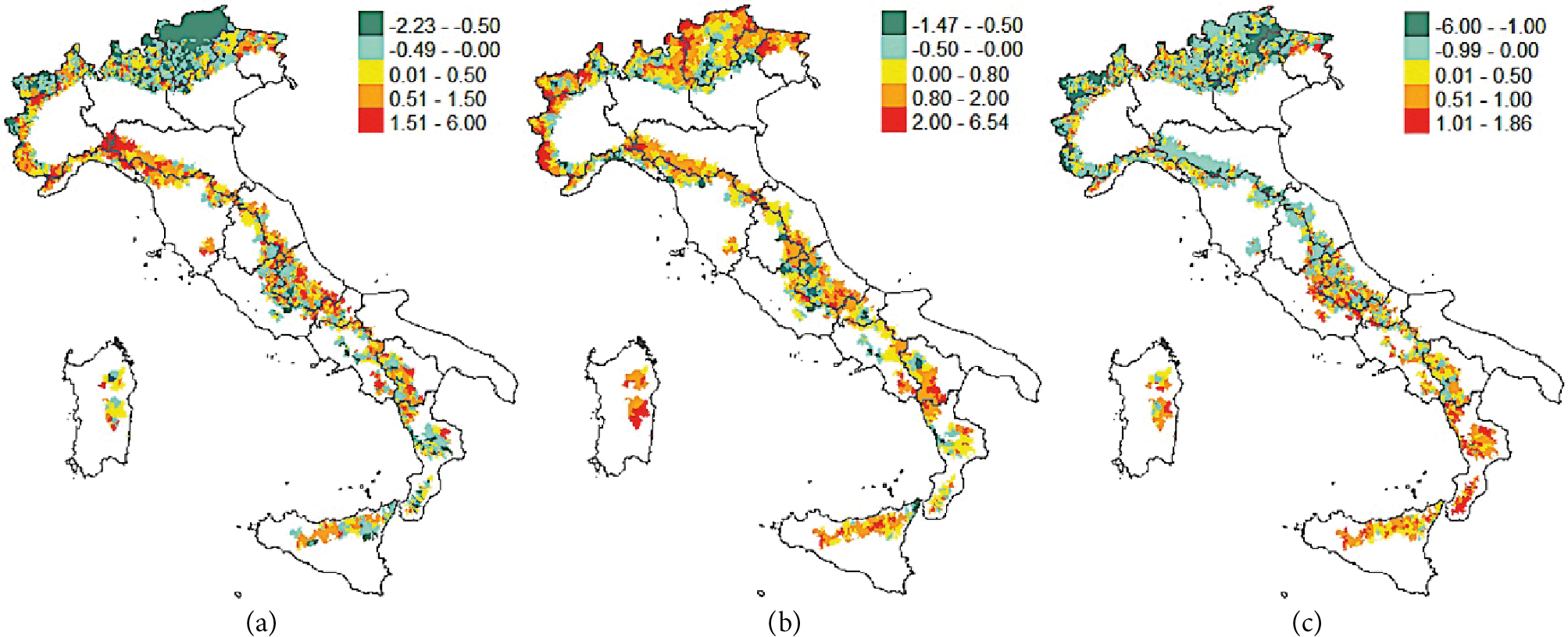
Table 7 shows the descriptive statistics of the independent variables in our ScaGWR model (1) by altimetric zone. Mountain areas present the highest medians for all three indexes, meaning that these areas are characterised by strong demographic, social, and economic weaknesses. The high SDs, especially for demographic and economic dimensions, indicate a certain amount of internal variability. Thus, mountain areas likely experience different scenarios.
| Altimetric zone | DWI | SDI | EWI | ||||||
|---|---|---|---|---|---|---|---|---|---|
| Median | Mean | SD | Median | Mean | SD | Median | Mean | SD | |
| Plain | -0.46 | -0.41 | 0.66 | -0.44 | -0.55 | 0.71 | -0.09 | -0.18 | 0.88 |
| Hill | -0.09 | 0.04 | 0.81 | -0.09 | -0.00 | 0.83 | 0.23 | 0.08 | 0.83 |
| Mountain | 0.12 | 0.30 | 1.11 | 0.58 | 0.46 | 0.70 | 0.26 | 0.05 | 1.01 |
| Italy | -0.15 | 0.00 | 0.93 | -0.09 | 0.00 | 0.85 | 0.14 | 0.00 | 0.91 |
Figure 2 displays the spatial distribution of the three aforementioned indexes in mountain areas. At a local scale, DWI and EWI exhibit a clear increasing gradient moving from northern to southern Italy (with a few exceptions for DWI in the most southern part of the country). There is much more widespread heterogeneity for SDI, which does not display any particular clusters but does show the presence of a majority of municipalities where essential services are absent.
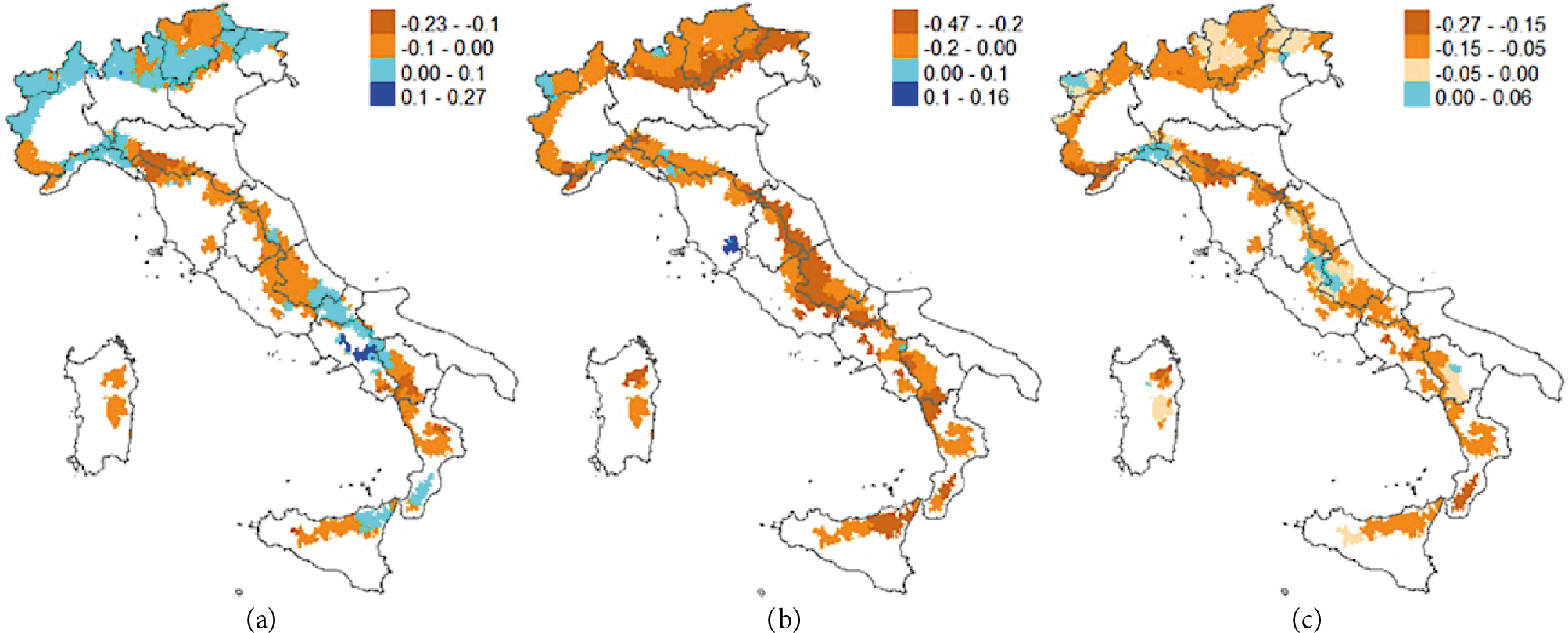
The most important calculation regarding the ScaGWR model involves the linear multiscale kernel defining the model weights, as shown in Equation (4). Thus, by defining as the median of the Q-nearest neighbour distances and following the algorithm proposed by Murakami et al. (2020), we set . For the two remaining parameters to be fixed in Equation (4), that is K (the maximum order of the polynomials) and Q (the number of neighbours), we tried different combinations and compared the results based on AICc and . The best combination was K = 3 and Q = 150. Figure 3 presents the main results for the estimated model (1). In particular, values for the parametric estimates of the single independent variables are displayed and only coefficients that are significant at the 5% level are shown.
In Figure 3a, the significant positive relationship linking DWI and SEVI is evident in many northern Italian municipalities. This could be due to the effect of the negative values expressing minor environmental vulnerability and the contextual negative DWI values present in the majority of these municipalities. This is the best possible combination because demographic vitality favours a healthy environment (Pilone, Demichela, 2018; Stotten et al., 2021). There is an exception in some parts of the Trentino-Alto Adige region: although SEVI and DWI have the same sign, the corresponding model coefficients are negative, suggesting that in this part of the country a favourable demographic status does not improve the state of the environment. Central Italy is characterised by a mainly inverse relationship between demographic weakness and environmental vulnerability. Most of the municipalities present a favourable environmental situation, indicating that they are experiencing depopulation and/or ageing phenomena. The estimated coefficients for southern Italy are mainly negative. However, it is worth noting the positive cluster between the Molise, Campania, and Basilicata regions, which is the result of the worst possible combination – have high values for both DWI and SEVI.
The map concerning SDI (Figure 3b) shows that almost all of the coefficients have a negative sign. remember that this indicates an inverse link between SDI and SEVI, apart from the algebraic values taken by the variables. Because the dependent variable, SEVI, is mostly lower than the mean, it follows that, as expected, rural and inner area municipalities are characterised by a higher SDI. This means that municipalities where essential services (health, education, and mobility) are lacking still exhibit a favourable environmental state.
Finally, the parametric estimates for EWI in Figure 3c indicate that there is a trade-off between economic activities and environmental state. Similarly to DWI, the Trentino-Alto Adige region stands out as a situation that is potentially very favourable, but this is not confirmed by the model results: the negative coefficient estimates do not seem to allow for good compatibility between the economy and the environment.
4. Discussion
Large portions of Italian mountain areas are characterised by social, economic, and demographic vulnerability. In terms of environmental vulnerability, apart from seismic and landslide risks, the overall environmental conditions are better thanks to the presence of vast wooded areas, extensive protected areas, lower atmospheric pollution, and less land consumption. These results reveal local diversity at a detailed administrative level, highlighting the role of a local approach to territorial vulnerability analysis (Shepherd, Dissart, 2022). This evidence reveals diversity at the local level on a detailed administrative scale, highlighting the need for a local approach to analysing territorial vulnerability. At a local level, there is some critical vulnerability in north-western Italy and, to a lesser extent, in some parts of central and southern Italy. In Piedmont, these vulnerabilities stem from demographic and environmental issues and the role of local mountain policies, which are characterised by deep fragmentation (Chilla et al., 2018). In both the southern Apennine areas and the Piedmont section, demographic and economic decline has been observed as confirmed by the recent Uncem (2025) report.
The results reveal strong demographic, social, and economic weaknesses. This dynamic can be explained by considering how population ageing is linked to less autonomy, with birth and mortality rates being an important element in classifying marginality (Cotella, Vitale Bovarone, 2020). Moreover, in Italy’s mountain areas there is a correlation between population loss, an increase in the number of elderly people, low income, and a general reduction in the supply of services (De Rossi, 2018). The positive relationship between DWI and SEFI in many municipalities in north-eastern Italy indicates a trade-off between lower environmental vulnerability and social demographic sustainability. In the central Apennines there is a positive environmental situation and a very worrying demographic situation. The mountains of southern Italy often present negative situations in terms of both environmental vulnerability and demographic weakness (Galderisi et al., 2022).
These elements are linked to economic aspects: depopulation and economic decline are highly correlated with distance to essential services (Camarero, Oliva, 2019). Furthermore, the number of enterprises and the level of employment are linked to the vitality of the local production system and rural development (Urso et al., 2019) and are useful for explaining the resilience of socio-economic systems in marginal areas (Faggian et al., 2018). The peripherality of mountain areas is linked to limited accessibility to essential services through a vicious circle of self-reinforcement, which negatively affects vulnerability (Cerea, Marcantoni, 2016). The difficult accessibility, distance from the main centres that provide essential services, increasing state of abandonment and degradation of the built heritage, and prevalence of the agricultural sector over other productive sectors contribute to explain the poor performance in socio-economic indicators, as discussed by De Rossi (2018). This framework has contributed to increasing marginality and a marked deterioration of social conditions, particularly in the mountain areas of southern Italy (Storti et al., 2020). These results seem to indicate a trade-off between the social and demographic fabric and environmental quality. While more intense land use might promote economic development, it might not be sufficient to prevent population loss and thus might have a negative impact on the provision of some ecosystem services (Vidal et al., 2013).
5. Conclusions
We investigated the environmental state of Italian mountain areas based on a synthetic vulnerability index and identified the socioeconomic drivers of such vulnerability at the local level. Rural development, agricultural planning, and environmental policies should consider the spatial distribution of vulnerability across mountain areas. Management policies that are more attentive to the characteristics of mountain areas are needed. Moreover, the relationship between environmental vulnerability and socio-economic structures must be analysed in depth – at the local level – to guide rural development and spatial planning policies, thus contributing to a more integrative and sustainable management of mountain areas. These systems require more effective governance models to combine environmental risk management with human activities.
Some limitations of the study need to be mentioned. We chose variables and adopted a synthetic index to incorporate the multifactorial, interactive, and spatial dimensions that characterise vulnerability in mountain areas. However, this also represents a critical issue related to the possibility of applying the model to different territorial contexts and to the limited availability of data at the municipal level, particularly economic data. From a methodological point of view, some limitations may arise from the possible conservative behaviour of GWR parametric estimators, which can lead to a very low rejection rate of the null hypothesis of no effect for local model variables.
Future research efforts can be made at the local level to investigate the causes and related aspects for the most vulnerable municipalities and the relationship between environmental vulnerability and the socioeconomic drivers. This could involve qualitative analysis, including multidisciplinary analysis. This is relevant for cases where there is low environmental vulnerability and good demographic, social, and economic conditions, such as the Trentino Alto Adige region. However, it is also crucial for regions for which we identified environmental vulnerability: the Apennine area (i.e., Basilicata) and in the north-western Alpine area, such as Piedmont.
Author Contributions
A.C.: Conceptualization, Investigation, Visualization, Writing – Original Draft, Writing – Review & Editing. G.C.: Supervision. L.M.: Conceptualization, Methodology, Investigation, Writing – Original Draft, Writing – Review & Editing. L.R.: Conceptualization, Methodology, Formal Analysis, Data Curation, Writing – Original Draft.
References
Acampora A., La Faci A., Leporanico V., Potenzieri M., Potenzieri M. (2023). Italian inner areas: demographic characteristics, employment and commuting and territorialdifferentiations. Rivista Italiana di Economia Demografia e Statistica, LXXVII, 1.
Acreman M., Hughes K.A., Arthington A.H., Tickner D., Duenas M.A. (2020). Protected areas and freshwater biodiversity: a novel systematic review distils eight lessons for effective conservation. Conservation Letters, 13(1). DOI: https://doi.org/10.1111/conl.12684.
Aroca-Jiménez E., Bodoque J.M., García J.A. (2020). How to construct and validate an integrated socio-economic vulnerability index: implementation at regional scale in urban areas prone to flash flooding. Science of Total Environment, 746, 140905. DOI: https://doi.org/10.1016/j.scitotenv.2020.140905.
Bankoff G., Hilhorst D. (2022). Why Vulnerability Still Matters: The Politics of Disaster Risk Creation. Routledge, London.
Bernués A., Tenza-Peral A., Gómez-Baggethun E., Clemetsen M., Eik L.O., Martín-Collado D. (2022). Targeting best agricultural practices to enhance ecosystem services in European mountains. Journal of Environmental Management, 316, 115255. DOI: http://doi.org/10.1016/j.jenvman.2022.115255.
Bordi I., Fraedrich K., Petitta M., Sutera A. (2007). Extreme value analysis of wet and dry periods in Sicily. Theoretical and Applied Climatology, 87: 61-71. DOI: https://doi: 10.1007/s00704-005-0195-3.
Bretagnolle V., Benoît M., Bonnefond M., Breton V., Church J., Gaba S., Lamouroux N. (2019). Action-orientated research and framework: insights from the French long- term social-ecological research network. Ecology and Society, 24(3): 10. DOI: https://doi.org/10.5751/ES-10989-240310.
Brooks N., Sethi R. (1997). The Distribution of Pollution: Community Characteristics and Exposure to Air Toxics. Journal of Environmental Economics and Management, 32(2): 233-250. DOI: https://doi.org/10.1006/jeem.1996.0967.
Callisto M., Solar R., Silveira F.A.O., Saito V.S., Hughes R.M., Fernandes G.W., Gonçalves-Júnior J.F., Leitão R.P., Massara R.L., Macedo D.R., Neves F.S., Alves C.B.M. (2019). A Humboldtian approach to mountain conservation and freshwater ecosystem services. Frontiers in Environmental Science, 7. DOI: https://doi: 10.3389/fenvs.2019.00195.
Camarero L., Oliva J. (2019). Thinking in rural gap: mobility and social inequalities. Palgrave Communications, 5: 95. DOI: https://doi.org/10.1057/s41599-019-0306-x.
Carrer F., Walsh K., Mocci F. (2020) Ecology, economy, and upland landscapes: socio-ecological dynamics in the Alps during the transition to modernity. Human Ecology, 48: 69-84. DOI: https://doi.org/10.1007/s10745-020-00130-y.
Cerea G., Marcantoni M. (2016). La montagna perduta. Come la pianura ha condizionato lo sviluppo italiano. FrancoAngeli, Milan.
Chilla T., Heugel A., Streifeneder T., Ravazzoli E., Laner P., Tappeiner U., Egarter L., Dax T., Machold I., Pütz M., Marot N., Ruault J.F. (2018). Alps 2050 common spatial perspectives for the Alpine area. Towards a common vision. Final Report, ESPON Project Targeted Analysis, ESPON EGTC, Luxembourg.
Cong Z., Feng G., Chen Z. (2023). Disaster exposure and patterns of disaster preparedness: a multilevel social vulnerability and engagement perspective. Journal of Environmental Management, 339, 117798. DOI: https://doi.org/10.1016/j.jenvman.2023.117798.
Cotella G., Vitale Bovarone E. (2020). Improving rural accessibility: a multilayer approach. Sustainability, 12, 2876. DOI: https://doi.org/10.3390/su12072876.
Cutter S.L. (2021). The changing nature of hazard and disaster risk in the Anthropocene. Annals of the American Association of Geographers, 111(3): 819-827. DOI: https://doi.org/10.1080/24694452.2020.1744423.
Cutter S.L., Ash K.D., Emrich C.T. (2014). The geographies of community disaster resilience. Global Environmental Change, 29: 65-77. DOI: https://doi.org/10.1016/j.gloenvcha.2014.08.005.
Dasgupta P. (2021). The Economics of Biodiversity: The Dasgupta Review. HM Treasury, London.
Dax T., Schroll K., Machold I., Derszniak-Noirjean M., Schuh B., Gaupp-Berghausen M. (2021). Land abandonment in mountain areas of the EU: an inevitable side effect of farming modernization and neglected threat to sustainable land use. Land, 10: 591. DOI: https://doi.org/10.3390/land10060591.
De Rossi A. (eds) (2018). Riabitare l’Italia. Le aree interne tra abbandoni e riconquiste. Donzelli, Rome.
Di Giovanni G. (2016). Post-earthquake recovery in peripheral areas: The paradox of small municipalities’reconstruction process in Abruzzo (Italy). Italian Journal of Planning Practice, VI: 110-139.
Drakes O., Tates E. (2022). Social vulnerability in a multi-hazard context: a systematic review. Environmental Research Letters, 17, 033001. DOI: https://doi.org/10.1088/1748-9326/ac5140.
Eckstein D., Künzels V., Schäfers L. (2021). Global Climate Risk Index 2021. GermanWatch, Berlin.
Esposito G., Salvatis P., Bianchis C. (2023). Insights gained into geo-hydrological disaster management 25 years after the catastrophic landslides of 1998 in southern Italy. International Journal of Disaster Risk Reduction, 84, 103440. DOI: https://doi.org/10.1016/j.ijdrr.2022.103440.
European Commission (2021). Overview of natural and man-made disaster risks the European Union may face: 2020 Edition, Publications Office of the European Union, Brussels. https://data.europa.eu/doi/10.2795/19072.
European Environment Agency (2020). Healthy environment, healthy lives: how the environment influences health and well-being in Europe, EEA Report n. 21/2019, Copenhagen.
Eurostat (2025). Rural Europe, European Commission, Luxembourg.
Faggian A., Gemmiti R., Jaquet T., Santini I. (2018). Regional economic resilience: the experience of the Italian local labor systems. The Annals of Regional Science, 60: 393-410. DOI: https://doi.org/10.1007/s00168-017-0822-9.
Ford J.D., Pearce T., McDowell G., Berrang-Ford L., Sayles J.S., Belfer E. (2018). Vulnerability and its discontents: the past, present, and future of climate change vulnerability research. Climatic Change, 151: 189-203. DOI: https://doi.org/10.1007/s10584-018-2304-1.
Fotheringham A.S., Brunsdon C., Charlton M. (2002). Geographically Weighted Regression: The Analysis of Spatially Varying Relationships. Wiley: New York.
Galderisi A., Bello G., Gaudio S. (2022). Le aree interne tra dinamiche di declino e potenzialità emergenti: criteri e metodi per future politiche di sviluppo. Archivio di Studi Urbani e Regionali, 133: 5-28.
Gariano S.L., Petrucci O., Rianna G., Santini M., Guzzetti F. (2018). Impacts of past and future land changes on landslides in southern Italy. Regional Environmental Change, 18: 437-449. DOI: https://doi.org/10.1007/s10113-017-1210-9.
Geldmann J., Barnes M., Coad L., Craigie I.D., Hockings M., Burgess N.D. (2013). Effectiveness of terrestrial protected areas in reducing habitat loss and population declines. Biological Conservation, 161: 230-238. DOI: https://doi.org/10.1016/j. biocon.2013.02.018.
Gobiet A., Kotlarski S. (2020). Future climate change in the European Alps. In Oxford Research Encyclopedia of Climate Science. Oxford University Press, Oxford. DOI: https://doi.org/10.1093/acrefore/9780190228620.013.767.
González-Leonardo M., Rowe F., Fresolone-Caparrós A. (2022). Rural revival? The rise in internal migration to rural areas during the COVID-19 pandemic. Who moved and Where? Journal of Rural Studies, 96: 332-342. DOI: https://doi.org/10.1016/j.jrurstud.2022.11.006.
IPCC (2023). Climate Change 2023: Synthesis Report. Contribution of Working Groups I, II and III to the Sixth. Assessment Report of the Intergovernmental Panel on Climate Change, Intergovernmental Panel on Climate Change, Geneva. DOI: https://doi.org/10.59327/IPCC/AR6-9789291691647.
Ispra (2018). Territorio. Processi e trasformazioni in Italia, Ispra Rapporti 296. Rome.
Ispra (2020). Rapporto rifiuti urbani, Ispra Rapporti 331. Rome.
Jha S.K., Negi A.K., Alatalo J.M., Negi R.S. (2021) Socio-ecological vulnerability and resilience of mountain communities residing in capital-constrained environments. Mitigation and Adaptation Strategies for Global Change, 26(8): 38. DOI: https://doi.org/10.1007/s11027-021-09974-1.
Karpouzoglou T., Dewulf A., Perez K., Gurung P., Regmi S., Isaeva A., Foggin M., Bastiaensen J., Van Hecken G., Zulkafli Z., Mao F., Clark J., Hannah D.M., Chapagain P.S., Buytaert W., Cieslik K. (2020). From present to future development pathways in fragile mountain landscapes. Journal of Environmental Science and Policy, 114: 606-613. DOI: https://doi.org/10.1016/j.envsci.2020.09.016.
Kokkoris I.P., Drakou E.G., Maes J., Dimopoulos P. (2018). Ecosystem services supply in protected mountains of Greece: setting the baseline for conservation management. International Journal of Biodiversity Science, Ecosystem Services and Management, 14: 45-59. DOI: https://doi.org/10.1080/21513732.2017.1415974.
Lenart-Boroń A.M., Boroń P.M., Prajsnar J.A., Guzik M.W., Żelazny M.S., Pufelska M.D., Chmiel M.J. (2021). COVID-19 lockdown shows how much natural mountain regions are affected by heavy tourism. Science of Total Environment, 806(3), 151355. DOI: https://doi.org/10.1016/j.scitotenv.2021.151355.
LeSage J.P. (2004). A family of geographically weighted regression models. In Anselin L., Florax R.J.G.M., Rey S.J. (eds) Advances in Spatial Econometrics. Advances in Spatial Science (pp. 241-264). Springer: Berlin, Heidelberg. DOI: https://doi.org/10.1007/978-3-662-05617-2_11.
Levers C., Schneider M., Prishchepov A.V., Estel S., Kuemmerle T. (2018). Spatial variation in determinants of agricultural land abandonment in Europe. Science of Total Environment, 644: 95-111. DOI: https://doi.org/10.1016/j.scitotenv.2018.06.326.
Lu B., Hu Y., Murakami D., Brunsdon C., Comber A., Charlton M., Harris P. (2022). High-performance solutions of geographically weighted regression. Geo-spatial Information Science, 25(4): 536-549. DOI: https://doi.org/10.1080/10095020.2022.2064244.
Marsden T. (2024). Contested ecological transitions in agri-food: emerging territorial systems in times of crisis and insecurity. Italian Review of Agricultural Economics, 79(3): 69-81. DOI: https://doi.org/10.36253/rea-15421.
Mastronardi L., Cavallo A., Romagnoli L. (2022). A novel composite environmental fragility index to analyse Italian ecoregions’ vulnerability. Land Use Policy, 122, 106352. DOI: https://doi.org/10.1016/j.landusepol.2022.106352.
Mottet A., Ladet S., Coque N., Gibon A. (2006). Agricultural land-use change and its drivers in mountain landscapes: a case study in the Pyrenees. Agriculture, Ecosystems and Environment, 114: 296-310.
Murakami D., Tsutsumida N., Yoshida T., Nakaya T., Lu B. (2020). Scalable GWR: a linear-time algorithm for large-scale geographically weighted regression with polynomial kernels. Annals of the American Association of Geographers, 111(2): 459-480. DOI: https://doi.org/10.1080/24694452.2020.1774350.
OECD (2022). States of Fragility 2022. OECD Publishing, Paris. DOI: https://doi.org/10.1787/c7fedf5e-en.
Pagliacci F., Luciani C., Russo M., Esposito F., Habluetzel A. (2021). The socioeconomic impact of seismic events on animal breeding. A questionnaire-based survey from central Italy. International Journal of Disaster Risk Reduction, 56, 102124. DOI: https://doi.org/10.1016/j.ijdrr.2021.102124.
Pagliacci F., Russo M. (2019). Multi-hazard, exposure and vulnerability in Italian municipalities. In Borsekova K., Nijkamp P. (eds.) Resilience and Urban Disasters (pp. 175-198). Edward Elgar Publishing: Cheltenham. DOI: https://doi.org/10.4337/9781788970105.00017.
Pilone E., Demichela M. (2018). A semi-quantitative methodology to evaluate the main local territorial risks and their interactions. Land Use Policy 77: 143-154. DOI: https://doi.org/10.1016/j.landusepol.2018.05.027.
Pirasteh S., Fang Y., Mafi-Gholami D., Abulibdeh A., Nouri-Kamari A., Khonsari N. (2024). Enhancing vulnerability assessment through spatially explicit modeling of mountain social-ecological systems exposed to multiple environmental hazards. Science of The Total Environment, 930, 172744. DOI: https://doi.org/10.1016/j.scitotenv.2024.172744.
Romano B., Zullo F., Fiorini L., Marucci A. (2021). “The park effect”? an assessment test of the territorial impacts of Italian National Parks, thirty years after the framework legislation. Land Use Policy, 100, 104920. DOI: https://doi.org/10.1016/j.landusepol.2020.104920.
Rumpf S.B., Gravey M., Brönnimann O., Luoto M., Cianfrani C., Mariethoz G., Guisan A. (2022). From white to green: snow cover loss and increased vegetation productivity in the European Alps. Science, 376(6597): 1119-1122. DOI: https://doi.org/10.1126/science.abn6697.
Shepherd P.M., Dissart J.C. (2022). Reframing vulnerability and resilience to climate change through the lens of capability generation. Ecological Economics, 201, 107556. DOI: https://doi.org/10.1016/j.ecolecon.2022.107556.
Schmeller D.S., Urbach D., Bates K., Catalan J., Cogălniceanu D., Fisher M.C., Friesen J., Füreder L., Gaube V., Haver M., Jacobsen D., Le Roux G., Lin Y., Loyau A., Machate O., Mayer A., Palomo I., Plutzar C., Sentenac H., Sommaruga R., Tiberti R., Ripple W.J. (2022). Scientists’ warning of threats to mountains. Science of Total Environment, 853, 158611. DOI: https://doi.org/10.1016/j.scitotenv.2022.158611.
Sena-Vittini M., Gomez-Valenzuela V., Ramirez K. (2023). Social perceptions and conservation in protected areas: Taking stock of the literature. Land Use Policy, 131, 106696. DOI: https://doi.org/10.1016/j.landusepol.2023.106696.
Stolton S., Dudley N., Avcıoğlu Çokçalışkan B., Hunter D., Ivanić K.-Z., Kanga E., Kettunen M., Kumagai Y., Maxted N., Senior J., Wong M., Keenleyside K., Mulrooney D., Waithaka J. (2015). Values and benefits of protected areas. In Worboys G.L., Lockwood M., Kothari A., Feary S., Pulsford I. (eds) Protected Area Governance and Management (pp. 145-166). ANU Press, Canberra.
Storti D., Provenzano V., Arzeni A., Ascani M., Silvia Rota F. (2020). Sostenibilità e innovazione delle filiere agricole nelle aree interne. Scenari, politiche e strategie. FrancoAngeli, Milan.
Stotten R., Ambrosi L., Tasser E., Leitinger G. (2021). Social-ecological resilience in remote mountain communities: toward a novel framework for an interdisciplinary investigation. Ecology and Society, 26(3): 29. DOI: https://doi.org/10.5751/ES-12580-260329.
Sun Y., Li Y., Ma R., Gao C., Wu Y. (2022). Mapping urban socio-economic vulnerability related to heat risk: a grid-based assessment framework by combing the geospatial big data. Urban Climate, 43, 101169. DOI: https://doi.org/10.1016/j.uclim.2022.101169.
Teare R. (2021). Reflections on the theme issue outcomes: Tourism sustainability in natural, residential and mountain locations: what are the current issues and questions? Worldwide Hospitality and Tourism Themes, 12(4): I-VI. DOI: https://doi.org/10.1108/WHATT-05–20200036.
Thorn J.P.R., Klein J.A., Steger C., Hopping K.A., Capitani C., Tucker C.M., Nolin A.W., Reid R.S., Seidl R., Chitale V.S., Marchant R. (2020). A systematic review of participatory scenario planning to envision mountain social-ecological systems futures. Ecology and Society, 25(3): 6. DOI: https://doi.org/10.5751/ES-11608-250306.
Tobler W.R. (1970). A computer movie simulating urban growth in the Detroit region. Economic Geography, 46: 234-240. DOI: https://doi.org/10.2307/143141.
Trigila A., Iadanza C. (2018). Landslides and floods in Italy: hazard and risk indicators - Summary Report, 267, Institute for Environmental Protection and Research (ISPRA). DOI: https://doi.org/10.13140/RG.2.2.14114.48328.
Uncem (2025). Rapporto Montagne Italia 2025. Istituzioni Movimenti Innovazioni. Le Green Community e le sfide dei territori, Rubettino, Soveria Mannelli.
UNDRO (1979). Natural Disasters and Vulnerability Analysis. Report of Expert Group Meeting, United Nations, Geneva.
UNISDR (2015). Sendai Framework for Disaster Risk Reduction, 2015-2030, United Nations, Geneva.
Urso G., Modica M., Faggian A. (2019). Resilience and sectoral composition change of Italian inner areas in response to the great recession. Sustainability, 11, 3432. DOI: https://doi.org/10.3390/su11123432.
Uval (2014). A strategy for inner areas in Italy: definition, objectives, tools and governance. Materiali Uval Series, Rome. http://www.dps.gov.it/it/pubblicazioni_dps/materiali_uval
Vendemmia B., Lanza G. (2022). Redefining marginality on Italian Apennines: An approach to reconsider the notion of basic needs in low density territories, Region, 9(2): 131-148. DOI: https://doi.org/10.18335/region.v9i2.430.
Vidal B., Martínez-Fernández J., Sánchez-Picón A., Pugnaire F. (2013). Trade-offs between maintenance of ecosystem services and socio-economic development in rural mountainous communities in southern Spain: A dynamic simulation approach. Journal of environmental management, 131. DOI: https://doi.org/10.1016/j.jenvman.2013.09.036.
Whitaker S.H. (2023). “The forests are dirty”: effects of climate and social change on landscape and well-being in the Italian Alps. Emotion, Space and Society, 49, 100973. DOI: https://doi.org/10.1016/j.emospa.2023.100973.