Research article
Sustainability and supply response of the sugarcane supply chain in Pakistan
Department of Agricultural and Food Sciences, University of Bologna, Italy
*Corresponding author. E-mail: zeeshanuaf@gmail.com
Abstract. Agricultural supply response is critical to economic development, particularly in a climate change scenario. This study uses a two-step generalised method of moments approach to examine the supply response of sugarcane to climatic and market factors in Pakistan from 1951 to 2010. The findings reveal a complex dynamic between cultivated area and yield, influenced by speculative behaviours, climatic conditions, regional research and development policies, and production factors. The results emphasise the importance of strategic resource allocation to mitigate climate impacts, develop drought-resistant varieties, subsidise farm inputs, enhance advisory services, and research and development funding to support sugarcane intensification and biodiversity protection.
Keywords: climate change adaptation, market dynamics, crop intensification, time series analysis.
JEL codes: Q01, Q13, Q16.
Index
3.2. Construction of the variables
4.2. Area and production trends
4.4. Elasticity of price and non-price factors
– Farmers’ crop and land decisions are highly responsive to price incentives.
– Policymakers must grasp supply responsiveness to avoid agri-food disruptions.
– The supply response of sugarcane in Pakistan highlights strategic resource allocation for sugarcane intensification and biodiversity.
The vulnerability and proneness of agri-food supply chains depend on the responsiveness of the dynamic agricultural production system (Edison et al., 2020; Gliessman, 2021), which may lead to food insecurity (Chavas et al., 2022), especially in a climate change scenario. These dynamic agricultural production systems are often estimated through agricultural supply response (ASR), that is, the acreage, yield, or output response to economic and/or non-economic incentives. Researchers have studied specific and/or isolated impacts of ASR – for example, output prices (Bor, Bayaner, 2009), input cost (Mustafa et al., 2016), and climate (Bassu et al., 2014; Chavas, Di Falco, 2017) – under specific policy settings (Lavanya, Manjunatha, 2025). ASR plays a central role in shaping farm design (Kalaiselvi et al., 2024) and agricultural policy (Doukas et al., 2022) to ensure sustainable and resilient agri-food supply chains.
In agricultural policy, prices influence farmers’ planning decisions regarding crop production and land use (Osborne, 2005). Low prices for farmers will discourage production, leading to food and primary input shortages that reduce economic development (Abrar et al., 2004). Price elasticity (the percentage rate of price changes) is mainly used for such policy evaluations, including support price and buffer stock operations, to estimate the demand/supply gap in agriculture (Haile et al., 2016). Therefore, within agri-food systems, the ASR of acreage and yield controls prices and bridges any demand/supply gaps for a crop (Nkang et al., 2007).
There are several complex, interconnected subsystems in agri-food systems in which key actors evolve dynamically. Each subsystem has unique features and behaviours that researchers must consider before developing models to ensure they obtain plausible estimates. (1) At the farm level, production is a dynamic phenomenon, and farmers are risk-averse (Antle, 1983), so it is necessary to include risk and price uncertainty (Chavas et al., 2022). (2) Each crop has a unique biological cycle, which requires consideration of crop- and location-specific characteristics. (3) It is necessary to include theoretically and mathematically sound/consistent indicators – for example, a clear differentiation among climate change (a decades-long and persistent long-term shift), climate variability (shorter-term fluctuations), and climate extremes (rare or unusually intense events). Moreover, technology is not linear, and its impact cannot be simplified by using time trends as a proxy for technological progress (Yu et al., 2018). (4) At the market level, the roles of buyers, intermediaries, and sellers are important within the existing marketing structure (Fligstein, Calder, 2015) as well as the prevailing government policies/regulations. Some researchers have already studied the problem in agricultural marketing, irrespective of ASR (Gohain, 2018; Skogstad, 1993). However, the limited data available means that these aspects are often overlooked in ASR research. As noted by Mbua, Atta-Aidoo (2023), there is a growing need for studies to inform policymakers about the drivers of agricultural supply chains and to provide a pathway for innovating agri-food systems.
Sugarcane – a crop highly sensitive to growing conditions – is a source of livelihood for around 100 million people worldwide (FAO, 2019). Pakistan is one of the top sugarcane producers in Asia, has the fastest annual population growth rate (1.9%), high per capita sugar consumption (24.64 kg), and an increasing trend in refined sugar imports (28,760 metric tons). Based on these factors, a recurring sugar crisis is looming (Pakistan Sugar Mills Association, 2021). The Government of Pakistan has implemented the Sugar Factories Control Act (1950) to regulate the sugarcane supply. This act established a sugarcane reservation area, restricting sugarcane growers’ options for selling their crop to only one designated mill and leaving no alternative buyers. Although the sugarcane zoning system was discontinued in 1987, new mills still experience barriers to entry. The millers (allegedly) collude with officials to circumvent loopholes (Pirzada et al., 2023), discouraging competition, increasing inefficiencies in ASR, and strengthening a monopsonistic regime (Alston et al., 1997).
The present study is designed to integrate multifaceted aspects of ASR related to sugarcane, the agricultural region, and climate change, and its responsiveness in the short and long run within one modelling framework via a two-step generalised method of moments with instrumental technique (GMM-IV). Our study is the first of its kind. We have attempted to include the following: (1) all important variables after robust theoretical consideration, such as climatic (change or variability) variables considering crop phenology, disaggregated drought estimates for climate extremes, and actual research and development (R&D) expenditures as a proxy for technological improvements; (2) the historical evolution of acreage and yield under government regulatory restrictions; and (3) a plausible estimation of total ASR (i.e., both acreage and yield responses). The estimates presented in this paper may be further improved based upon the availability of data from the year 2010 onwards, including data on agricultural-marketing-related problems (e.g., delays in procurement [crushing season], the length of the crushing season, the wait time for weighing and unloading, a deduction in payments, and the timing of announcement of crop support price, among other factors).
The remainder of the article is organised as follows. Section 2 provides a literature review that highlights the importance of sugarcane within the agri-food system and the rationale for this research. Section 3 introduces the data selected, the construction of the derived variables, and the statistical analysis. Section 4 covers the results and discussion, and Section 5 summarises the main findings and policy implications. In the rest of this paper, we have used some terms interchangeably: cultivated area for acreage or crop area; agricultural production region for region or district; and climate dynamics for climate change as a whole (long-term gradual change), climate variability (short-term abrupt changes), and climate extremes or shocks (rare or unusual incidents).
The ASR literature has two distinct streams. The first stream is dominant and related to crop duration: annual (Abrar et al., 2004; Lobell et al., 2013, 2014) or perennial (Devadoss, Luckstead, 2010; Wani et al., 2015). Researchers have also considered risks and uncertainty (Antle, 1983). Price volatility is the primary source of uncertainty (Mustafa et al., 2024); it affects both productivity – technical efficiency (Đokić et al., 2022) and optimal resource use – and allocative efficiency (Mivumbi, Yuan, 2023) and, hence, overall economic efficiency (Chen et al., 2023). The second stream has focused on devising a sophisticated methodological framework to obtain plausible estimates (Elnagheeb, Florkowski, 1993; Mearns et al., 1997; Mendelsohn et al., 1994). However, the estimates are not consistent or robust, so it is necessary to systematically integrate the climate, crop, and economic results from different types of models. Results from crop- and location-specific models (Ray et al., 2012) can be integrated to assess the resilience of the agroeconomic system to climate change (Chavas, Di Falco, 2017; Nelson et al., 2014) and to better understand its underlying marketing structures.
There have been few studies on the responses of field crops to gradual climate changes at a decadal scale. Several researchers have investigated the impacts of seasonal climate variability on crop production (Chen, Chang, 2005; Tao et al., 2006). The effects of extreme events, such as drought, are often ignored and/or aggregated, leading to a failure to depict ground-level water conditions. These climate extremes also affect farmers’ expectations and risk perceptions throughout a crop cycle (Yu et al., 2021). Other studies have excluded key variables such as prices, which are important to capture the cyclical behaviour over time (Von Cramon-Taubadel, Goodwin, 2021), the irrigated land share (Hertel, 2011), fertiliser consumption (Boansi, 2014), and the biological cycle of crops (Devadoss, Luckstead, 2010). These omissions may result in implausible or even biased estimates (Alston, Chalfant, 1991).
In Pakistan, there is a dearth of research on sugarcane. The first reported study on sugarcane acreage response included only the relative price index, based on 28 years of time-series data (from 1915-1916 to 1943-1944), from the undivided Punjab region of India and Pakistan (Krishna, 1963). Ali (1990) included sugarcane in evaluating production supply response, but only with respect to fertiliser price. Wasim (1997) focused on the response of sugarcane (irrigated acreage) to price and yield risk, along with plant protection measures and sugar production, based on 21 years of data (from 1972-1973 to 1993-1994) from five districts of the Sindh province. Mushtaq, Dawson (2002) examined the response of sugarcane acreage to wholesale prices, irrigated area, and sowing-season rainfall using 36 years of data (1960-1996) from Pakistan. Shafique et al. (2007) analysed the supply response of acreage and yield to the crop’s own price, the cotton price, canal water availability at sowing, fertiliser prices, and rainfall during the sowing period, based on 32 years of data (1970-2001) from various agro-ecological zones in Punjab. At the country level, Khan, Hussain (2007) studied the sugarcane acreage response to the support price, water availability, and yield using 18 years of data (from 1985-1986 to 2003-2004), while Nosheen, Iqbal (2008) estimated acreage response to sugarcane price and yield only, based on 36 years of data (1970–1971 to 2006-2007). Yaseen, Dronne (2011) estimated the response of sugarcane output (gross product per hectare) to the sugarcane area, price, and yield using only 42 years of data (1966-2008). Saddiq et al. (2013) studied the response of sugarcane crop area to prices, yield, and rainfall using 42 years of data (1970-2011) from the North West Frontier Province (now called Khyber Pakhtunkhwa [KP]).
The synthesis of previous research from Pakistan raises serious concerns about the plausibility of ASR estimates. To date, the long-term climate dynamics for sugarcane have not been empirically quantified with advanced methods. When modelling dynamic production systems, endogeneity often poses a serious challenge, making ordinary least squares estimates unreliable. To address this issue, robust estimators that are consistent in the presence of heteroscedasticity and autocorrelation – such as those obtained with the GMM-IV model – are more appropriate. However, most previous studies have relied on low-frequency, aggregated data at the national or provincial level. High-frequency panel data, by contrast, can reveal significant differences between micro- and macro-level supply responses (Wu, Adams, 2002). Aggregating parameters across broader geographic areas (e.g., from district to province) alters their underlying distributions and reflects different market and policy environments. In addition, earlier studies have rarely accounted for sugarcane’s biological cycle or technological changes, both of which are crucial for accurate estimation. These omissions can distort the representation of macro-level dynamics and lead to biased or inconclusive results (Hannay, Payne, 2022). In ASR analysis involving acreage, it is essential to understand the historical evolution of cultivated area and yield (Babcock, 2015) before quantifying their roles within agri-food systems. Therefore, it is necessary to revisit ASR analysis using high-frequency, crop- and location-specific data to generate more concrete insights into the resilience and sustainability of Pakistan’s sugarcane supply chain.
We performed a descriptive analysis to understand the historical evolution of the cultivated area and yield; it involves a description of farm management and land use under prevailing climatic and marketing conditions. We performed an empirical analysis to estimate and revalidate ASR for the sugarcane crop at the district level.
We quantified the behaviour of the farmers’ decision variable(s) by using the Nerlovian reduced-form model (Ngoc et al., 2022). This model has the advantage of capturing the speed of adjustment and the rate of change in the response variable. In this model, let Bt be the dependent variable and Zt be the vector of regressors, including price and non-price factors. The Nerlovian reduced-form model distinguishes between the actual level of the variable, Bt, and the desired level, , which the farmer aims to achieve based on the values of the decision variables (Equation 1).
(1)
The actual level then adjusts towards this level, according to Equation (2):
(2)
where is the speed adjustment to the desired level. This means that the change in any given period is proportional to the gap between the actual and desired levels in the previous period (i.e., ), so our model is dynamic (Tenaye, 2020). When this parameter is close to zero, adjustment is slow, while a high value indicates fast adjustment.
For the present study, we specifically derived Equations (3) and (4) for the current sugarcane cultivated area (At in 000 ha) and yield (Yt, in tons/ha) responsiveness in the ith districts.
(3)
(4)
where P is the price of produce and fertilisers (cost), Z is an array of exogenous variables (non-price factors), (α0, β0) is the offset parameter, and (µit, ϑit) are the noise components. α and β are short-run elasticities with respect to price and non-price factors for the cropped area and yield, respectively.
All variables are expressed in the logarithmic form (e.g., A' = log A), while allowing the total production (TP’) response to be expressed in logarithmic terms as a sum of the area and yield responses (TP' = A' + Y'). When the area ( ) and yield ( ) elasticities are higher, farmers who cultivate sugarcane make faster adjustments (Wang et al., 2020).
We also hypothesise that growers are rationally efficient (Liu et al., 2016) and all long-run elasticities exceed the short-run elasticities (Tenaye, 2020). Farmers quickly adjust their cultivated area to the desired level if the adjustment coefficient is close to 1 and vice versa. In addition, the presence of lagged dependent variables can lead to autocorrelation. The two-step GMM-IV model (Baum et al., 2003) is appropriate if the error distribution is not independent of the distribution of the regressors. We used the GMM-IV model to compute the area and yield response estimates to ensure robust homoscedasticity and autocorrelation consistency while treating lagged dependent and price variables as predetermined (i.e., instruments).
3.2. Construction of the variables
We considered sugarcane fertiliser uptake and diammonium phosphate (DAP) prices as essential farm inputs and precipitation/temperature as essential climatic variables (Chavas et al., 2019). Because sugarcane is sensitive to conditions at each stage of growth, we computed a 30-year rolling average of climatic variables for each growth stage (He et al., 2020; Rezaei et al., 2018). In other words, the climatic variables computed for 1981 are the average of the previous 30 years (1951–1980), and the same approach is applied for the other variables and times (Van Der Wiel, Bintanja, 2021). We considered the sample from 1981 to 2010 for further analysis.
To characterise the variability and distribution of climatic conditions, we calculated the coefficients of variation (climate anomalies) for monthly precipitation and temperature, accounting for the sugarcane growth stages. We identified four key stages based on consultations with national sugarcane experts in Pakistan (personal communications) and the literature (Thornton et al., 2014): sowing and germination (January-March), tillering (April-June), grand growth (July-August), and maturity and harvesting (September-November). Given the importance of drought in influencing the area and yield responses in water-scarce districts (Shehzad et al., 2022), we computed the Pálfai Drought Index (PaDI) using Equation (5) to quantify the impact of extreme events at the district level (Jahangir, Danehkar, 2022).
(5)
where PaDI0 is the base value of the drought index (°C/100 mm), Ti is the monthly mean temperature from April to August (°C), Pi is the monthly sum of precipitation from September to October (mm), wi is a weighting factor, and is a constant (10 mm).
We based the analyses on a monthly time series from 1951 to 2010 from 20 leading sugarcane-producing districts in Pakistan. After 2010, several new districts were created, and their historical data became unavailable. Therefore, the final sample was restricted to 2010.
We considered districts with sufficiently high sugarcane production (>5% share in national sugarcane production) and the availability of meteorological observations and the existence of a district from the 1950s (Hazrana et al., 2020). Based on these criteria, we selected nine districts from Punjab, eight from Sindh, and eight from KP. The Pakistan Bureau of Statistics (PBS) provides district-level data on area, yield, total macronutrient uptake (NPK nutrients), crop prices, and fertilisers. The National Agricultural Research Centre (NARC) in Islamabad, Pakistan, provides the R&D expenditures. The Pakistan Meteorological Department (PMD) provides district-level data on climatic variables. Table 1 reports the variables and their sources, including the derived variables.
| Variable | Description | Units (estimation) | Sources | ||||||||||||||||
|---|---|---|---|---|---|---|---|---|---|---|---|---|---|---|---|---|---|---|---|
| A | Sugarcane cultivated area | (× 1000) hectares | PBS | ||||||||||||||||
| Y | Sugarcane yield | ton/ha | |||||||||||||||||
| *Prices and costs | |||||||||||||||||||
| CP | Cotton | PKR/40 kg | |||||||||||||||||
| MP | Maize | ||||||||||||||||||
| RP | Rice | ||||||||||||||||||
| SP | Sugarcane | ||||||||||||||||||
| WP | Wheat | ||||||||||||||||||
| DAP | Diammonium phosphate | PKR/50 kg | |||||||||||||||||
| Inputs | |||||||||||||||||||
| TNU | Total nutrient uptake | NPK kg/hectares | National Fertilizer Development Centre (NFDC) | ||||||||||||||||
| NU | Nitrogen uptake | kg/hectares | |||||||||||||||||
| PU | Phosphorus uptake | ||||||||||||||||||
| KU | Potassium uptake | ||||||||||||||||||
| PK | Phosphorus/potassium nutrient ratio | Index | Own calculations | ||||||||||||||||
| PNPK | Phosphorus/total nutrient ratio | ||||||||||||||||||
| PN | Phosphorus/nitrogen nutrient ratio | ||||||||||||||||||
| PIC | Irrigated overcultivated area ratio | ||||||||||||||||||
| R&D | Research and development expenditures | PKR (millions) | NARC | ||||||||||||||||
| Climate | |||||||||||||||||||
| Prec. | Average rainfall | Moving average (mm) | PMD | ||||||||||||||||
| Temp. | Average temperature | Moving average (°C) | |||||||||||||||||
| PG | Precipitation at germination | Average (mm) | Own calculations | ||||||||||||||||
| PT | Precipitation at tillering | ||||||||||||||||||
| PGG | Precipitation at grand growth | ||||||||||||||||||
| PM | Precipitation at maturity | ||||||||||||||||||
| PS | Precipitation shocks | Index | |||||||||||||||||
| PSG | Precipitation shocks at germination | ||||||||||||||||||
| PST | Precipitation shocks at tillering | ||||||||||||||||||
| PSGG | Precipitation shocks at grand growth | ||||||||||||||||||
| PSM | Precipitation shocks at maturity | ||||||||||||||||||
| TG | Temperature at germination | Average (°C) | |||||||||||||||||
| TT | Temperature at tillering | ||||||||||||||||||
| TGG | Temperature at grand growth | ||||||||||||||||||
| TM | Temperature at maturity | ||||||||||||||||||
| TS | Temperature shocks | Index | |||||||||||||||||
| TSG | Temperature shocks at germination | ||||||||||||||||||
| TST | Temperature shocks at tillering | ||||||||||||||||||
| TSGG | Temperature shocks at grand growth | ||||||||||||||||||
| TSM | Temperature shocks at maturity | ||||||||||||||||||
| PaDI | Pálfai Drought Index | Index | Jahangir, Danehkar, 2022 | ||||||||||||||||
| Notes: In actual model estimations, we have used real crop and fertilisers prices after deflating wtih consumer price index (CPI), retrieved from the World Bank. All variables were used in the logarithmic form except for drought. Note that TNU considers the use of nitrogen, phosphorus, and potassium fertilisers. | |||||||||||||||||||
Our analysis shows that the farmers’ allocation decisions result in significant variations in the sugarcane-cultivated area and yield. In Sindh, the area is around 40,000 ha, and the yield is around 14 tons/ha (Table 2). These values for this province have been ascribed to the appearance of new sugar mills, a favourable environment for cultivation, and improved technical and allocative efficiency of farmers from 1981 to 2010 (Khushk et al., 2011).
| Variable | KP | Punjab | Sindh | ||||||||||||||||
|---|---|---|---|---|---|---|---|---|---|---|---|---|---|---|---|---|---|---|---|
| Mean | SD | Mean | SD | Mean | SD | ||||||||||||||
| A | 30.03 | 18.17 | 57.27 | 32.72 | 40.51 | 39.78 | |||||||||||||
| Y | 41.85 | 6.77 | 42.32 | 6.92 | 46.67 | 13.44 | |||||||||||||
| TNU | 582.65 | 452.02 | 913.36 | 1533.25 | 1341.98 | 986.64 | |||||||||||||
| CP | 851.75 | 288.77 | 851.75 | 288.15 | 851.75 | 288.25 | |||||||||||||
| MP | 315.83 | 87.69 | 316.60 | 82.37 | 319.93 | 79.56 | |||||||||||||
| RP | 672.45 | 714.05 | 672.45 | 710.05 | 672.45 | 710.30 | |||||||||||||
| SP | 45.66 | 28.33 | 45.30 | 28.03 | 46.07 | 28.31 | |||||||||||||
| WP | 391.70 | 277.26 | 391.70 | 275.70 | 391.70 | 275.80 | |||||||||||||
| DAP | 869.23 | 645.00 | 869.23 | 641.39 | 869.23 | 641.61 | |||||||||||||
| PaDI | 4.83 | 2.02 | 11.02 | 6.04 | 6.74 | 6.91 | |||||||||||||
| PS | 7.00 | 1.41 | 6.86 | 3.00 | 5.52 | 2.39 | |||||||||||||
| TS | 1.99 | 0.59 | 2.59 | 0.25 | 3.05 | 0.51 | |||||||||||||
| PIC | 1.16 | 0.44 | 0.94 | 0.35 | 0.70 | 0.31 | |||||||||||||
| PKR. | 54.76 | 68.16 | 38.65 | 69.05 | 24.31 | 20.72 | |||||||||||||
| PNPK | 0.19 | 0.06 | 0.18 | 0.05 | 0.18 | 0.04 | |||||||||||||
| PN | 0.24 | 0.11 | 0.229 | 0.08 | 0.24 | 0.12 | |||||||||||||
| Prec. | 40.95 | 13.72 | 34.76 | 18.43 | 15.54 | 8.60 | |||||||||||||
| Temp. | 22.33 | 2.28 | 25.65 | 1.56 | 27.51 | 1.21 | |||||||||||||
| R&D | 0.20 | 0.23 | 14.20 | 10.91 | 2.04 | 3.00 | |||||||||||||
| Notes: See Table 1 for a description of each variable. For simplicity, the interactions of the climactic variables (Temp. and Prec.) with crop phenology have been omitted. | |||||||||||||||||||
There is a skewed, intermittent distribution of R&D expenditures across provinces. From 1981 to 2010, the highest R&D expenditure was in Punjab (around 14 million) and the lowest in KP (0.20 million).
The highest annual precipitation was in KP (41 mm), and the highest monthly mean temperature was in Sindh (28°C). Although the average temperature is almost equal to the optimal value for sugarcane (27°C; Ebrahim et al., 1998), there are considerable variations throughout the sugarcane crop cycle. Precipitation and temperature variability are more pronounced in KP (12 points) and Sindh (5 points). In contrast, the coefficients of variation of precipitation and temperature shocks are higher in Sindh (125%) than in KP (40%).
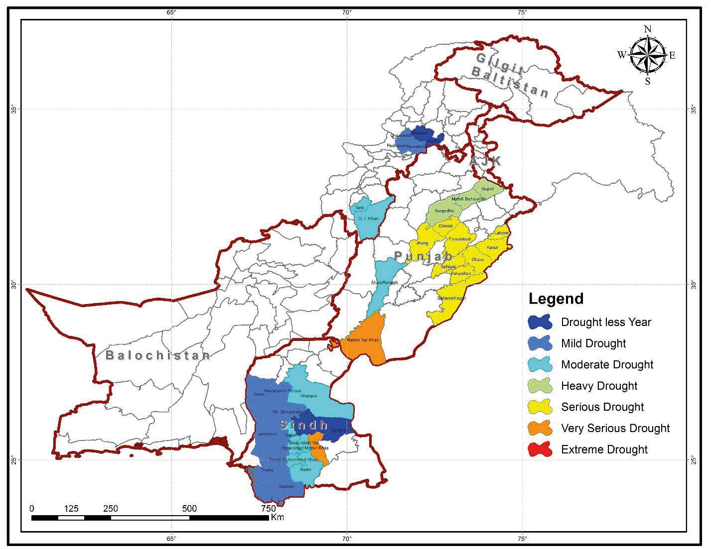
There has been a severe drought-like situation in Punjab, compared with Sindh (moderate drought) and KP (mild drought), across the sugarcane-producing districts (Figure 1). This situation is another reason for KP’s high natural potential for sugarcane production, compared to Punjab.
4.2. Area and production trends
Figure 2 presents the sugarcane cultivated area and production from 1981 to 2010. The changes over time reflect the growers’ choices and cropland planning. The only district to show significant growth in sugarcane-cultivated land is D.I. Khan in KP. These increases in cropland result from adjustments in cropping patterns or the occupation of pristine land, especially in the D.I. Khan district. The recent study by Hussain, Khan (2021) supports our results, as they reported a higher deforestation rate in the D.I. Khan district.
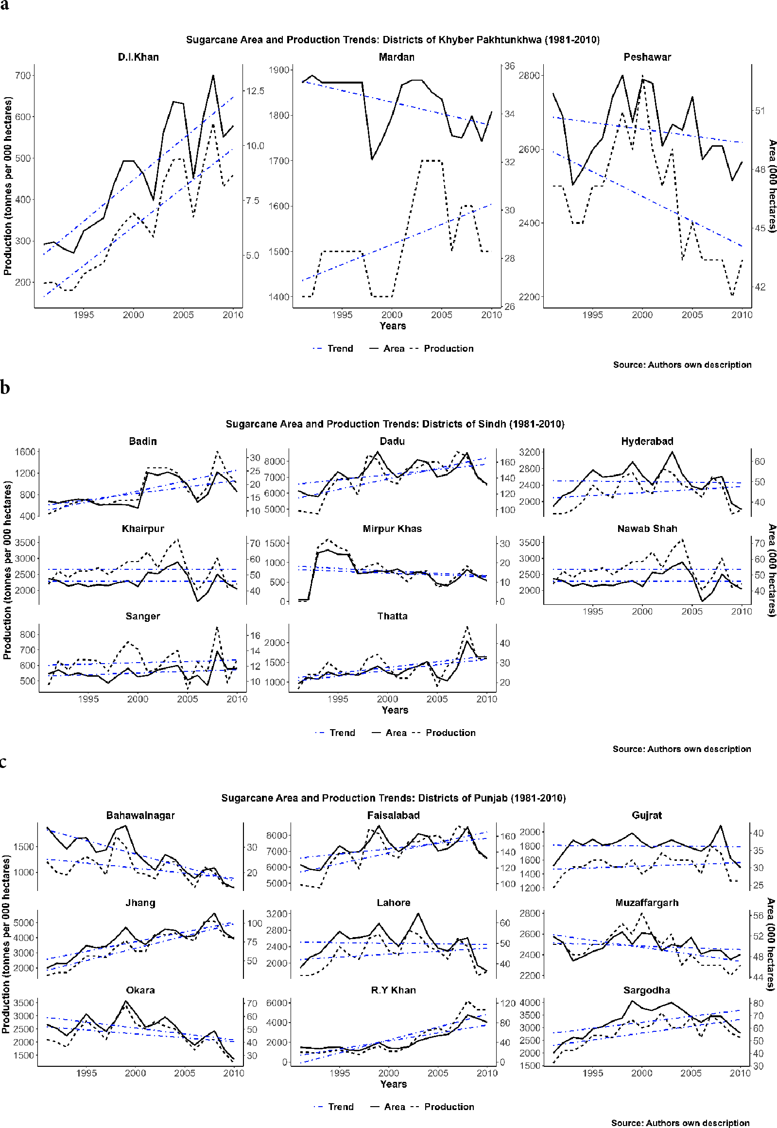
During 1999-2000, there were spikes in production in five districts: Peshawar in KP; Muzaffargarh in Punjab; and Mirpur Khas, Sanger, and Thatta in Sindh. During this time, the recorded production harvested led to a domestic surplus in the sugarcane supply, despite a reported 13% reduction in cultivated area. The boom cycle ended within the next three years; as a result, sugar prices remained stagnant (Pakistan Sugar Mills Association, 2000). Production offset the trend of increased cultivated area in the Gujrat, Lahore, and Sargodha districts, especially in 2004-2005.
The reason for such trends can be attributed to different growth rates in cultivated area (0.4%) and yield (2.9%), and to an increase in sugarcane price support (1.5 times from 2005 to 2010) in Punjab (USDA-FAS, 2021). In the Bahawalnagar district (Punjab), farmers have exchanged land for more profitable crops, such as rice, resulting in a drastic decrease in acreage. Overall, the results indicate no uniform relationship across the districts. Farmers are making quick adjustments in area allocation and optimising farm inputs as mitigation and adaptation strategies to offset the negative impacts of climate change.
This section focuses on understanding the magnitude and speed of technological adjustments (Table 3). We used the under-identification (p < 0.05), weak identification (F = 1742.677), and over-identification (p > 0.05) tests to validate the results.
| Variable | Area (× 1000 hectares) |
Yield (tonnes per hectare) |
Variable | Area (× 1000 hectares) |
Yield (tonnes per hectare) |
||||||||||||||
|---|---|---|---|---|---|---|---|---|---|---|---|---|---|---|---|---|---|---|---|
| β ± standard error | β ± standard error | β ± standard error | β ± standard error | ||||||||||||||||
| R&D | 0.014 ± 0.017 | -0.127 ± 0.072** | A (t-1) | 0.936 ± 0.020*** | - | ||||||||||||||
| PIC | 0.050 ± 0.026** | -0.084 ± 0.094 | Y (t-1) | - | 0.565 ± 0.062*** | ||||||||||||||
| PK | -0.016 ± 0.009* | -0.016 ± 0.019 | PN | 0.250 ± 0.143* | 0.270 ± 0.538 | ||||||||||||||
| TT | -0.465 ± 0.192** | 0.257 ± 0.792 | PNPK | -0.193 ± 0.106* | -0.230 ± 0.398 | ||||||||||||||
| TGG | 0.837 ± 0.292*** | -0.594 ± 0.975 | Constant | -0.339 ± 0.120*** | 0.146 ± 0.317 | ||||||||||||||
| TM | -0.435 ± 0.227* | 0.509 ± 0.825 | PT2 | 0.202 ± 0.069*** | 0.059 ± 0.142 | ||||||||||||||
| PSGG | 0.387 ± 0.115*** | -0.859 ± 0.624 | TGG2 | 0.081 ± 0.048* | -0.180 ± 0.132 | ||||||||||||||
| PSM | 0.506 ± 0.222** | -0.216 ± 0.506 | TSG | -0.302 ± 0.174* | 0.346 ± 0.760 | ||||||||||||||
| TG × PG | -0.148 ± 0.218 | 0.934 ± 0.560* | TST | 0.107 ± 0.051** | 0.016 ± 0.131 | ||||||||||||||
| TT × PT | 0.135 ± 0.076* | -0.068 ± 0.253 | CP | 0.090 ± 0.039** | 0.360 ± 0.117*** | ||||||||||||||
| TGG × PGG | 0.102 ± 0.049** | -0.247 ± 0.109** | RP | 0.140 ± 0.043*** | -0.006 ± 0.156 | ||||||||||||||
| DAP | -0.085 ± 0.052 | -0.285 ± 0.142** | SP | -0.264 ± 0.076*** | -0.013 ± 0.181 | ||||||||||||||
| DAP × CP | -0.133 ± 0.058** | -0.661 ± 0.208*** | DAP × SP | 0.225 ± 0.082*** | 0.467 ± 0.235** | ||||||||||||||
| DAP × RP | -0.286 ± 0.067*** | -0.330 ± 0.163** | DAP × WP | 0.126 ± 0.113 | 0.420 ± 0.246* | ||||||||||||||
| Area | Yield | ||||||||||||||||||
| Observations | 380 | 380 | |||||||||||||||||
| Under-identification test | |||||||||||||||||||
| Kleibergen-Paap rk LM statistic | 42.912*** | 55.735*** | |||||||||||||||||
| Weak identification test | |||||||||||||||||||
| Cragg-Donald Wald F statistic | 1742.677NS | 1696.233NS | |||||||||||||||||
| Over-identification test | |||||||||||||||||||
| Hansen J statistic (p-value) | 0.237 | 0.409 | |||||||||||||||||
| F-test for joint significance (p-value) | 0.000 | 0.000 | |||||||||||||||||
| Note: See Table 1 for a description of each variable. All variables are standardised before deflating the price series (crops and fertilisers) with the consumer price index. The reported standard errors are robust to heteroskedasticity and autocorrelation. The coefficients are two-step GMM-IV estimates, including the lagged dependent variable and predetermined price variables. The results for non-significant terms are omitted: A (for yield only), and PaDI, PG, PT, PGG, PM, TG, PSG, PST, TPG, TPM, PGG2, PM2, TG2, TT2, TM2, TSGG, TSM, MP, WP, and DAP × MP (for area and yield). The asterisks indicate statistical significance: ***p < 0.01, **p < 0.05, and *p < 0.1. NS means not significant. | |||||||||||||||||||
The lagged coefficient is higher for the area than for the yield (0.94 vs 0.57), which agrees with the outcomes described in the previous section (Table 3). The higher sugarcane production may be attributed to horizontal expansion (which can be related to the imperfections of the market). The adjustment coefficients for the area and year are <1, indicating a slow adjustment in the long-run equilibrium. The current pace of the farmers’ decisions is expected to bring the yield back to equilibrium in approximately 2.3 years in the case of an unexpected (price and non-price) shock.
We addressed the sugarcane supply-climate change nexus using linear and nonlinear parameterisations of climatic variables. Precipitation shocks at grand growth (0.39%) and maturity (0.51%) resulted in positive shifts, as indicated by a combined increase of 900 ha in sugarcane area allocation. A pronounced (non-linear) impact of precipitation at the tillering stage resulted in a 0.20% increase (an additional 200 ha) from 1981 to 2010. Optimal rainfall is crucial for a higher number of tillers and thus a higher sugarcane yield (Vasantha et al., 2012).
The cultivated area is more responsive to the linear temperature changes than to its non-linear fluctuations. There is an increase of approximately 470 ha in sugarcane land due to a 1% increase in temperature at the tillering stage. In contrast, temperature at the grand growth stage shows a parabolic pattern, as indicated by the significant squared term in the model (i.e., TGG2). The temperature increases linearly at the maturity stage and has a significant negative (-0.44%) short-run elasticity, resulting in a 440-ha decrease in the sugarcane-cultivated area (de Medeiros Silva et al., 2019).
The average temperature in our sampling framework during this stage was 25°C, whereas the optimum temperature for sucrose accumulation at maturity is 12-14°C (Verma et al., 2019). The long-term implications of these results include changes in production (food availability), disruptions in food volume, and alterations in trade patterns in domestic and international markets (Santeramo et al., 2021).
It appears that R&D expenditure significantly (and adversely) affects the yield response, with a short-run elasticity of -0.13%. In Pakistan, R&D investment in cereals has been higher than in sugarcane. Most R&D expenditure has focused on maintaining sugarcane yield rather than enhancing it (Abraham, Pingali, 2021). These results highlight the uncertainty that arises from underinvestment in R&D (Pardey et al., 2006) and imperfect market conditions (Mai, Lin, 2021), questioning the validity of previous computed results.
Regarding the farm inputs, the short-run elasticity of the P:N ratio is 0.25%, resulting in a higher area response than the P:K ratio (-0.02%) and the P:NPK ratio (-0.19%), decreasing the sugarcane area response. This result indicates that the imbalance in fertiliser use stems from the use of potassium nutrients, which may reduce the sugarcane crop area. These imbalances can be ascribed to a lack of subsidies and increasing prices (Ali et al., 2016).
According to economic theory, we should expect important effects from complementary crops (Santeramo et al., 2021). The cotton price has significant positive short-run elasticities for area (0.09%) and yield (0.36%). Specifically, growers are unable to convert the area used to cultivate sugarcane to area used to cultivate cotton, as the sowing time overlaps with sugarcane (starting in mid-February). The yield response to cotton prices is higher, as sugarcane farmers could earn higher profits in September from conventional cotton harvesting. Farmers can purchase inputs used to grow sugarcane on time, just before the crop matures.
The relationship between sugarcane price and area (yield) is negative, in contrast to standard production theory (Yu et al., 2012). The growers reallocate only around one-fourth of their desired level within 1 year as their price elasticity is -0.26%. This could be attributed to delayed or reduced payments by sugar mills compared with the announced prices. The beginning of the late cane-crushing season is another important factor. These adjustments are further exacerbated by increased DAP prices and an additional 0.09% reduction in the sugarcane area in the short run. The impacts of increased DAP prices are more pronounced in the yield response, with approximately a 30% reduction in yield accounting for these price surges.
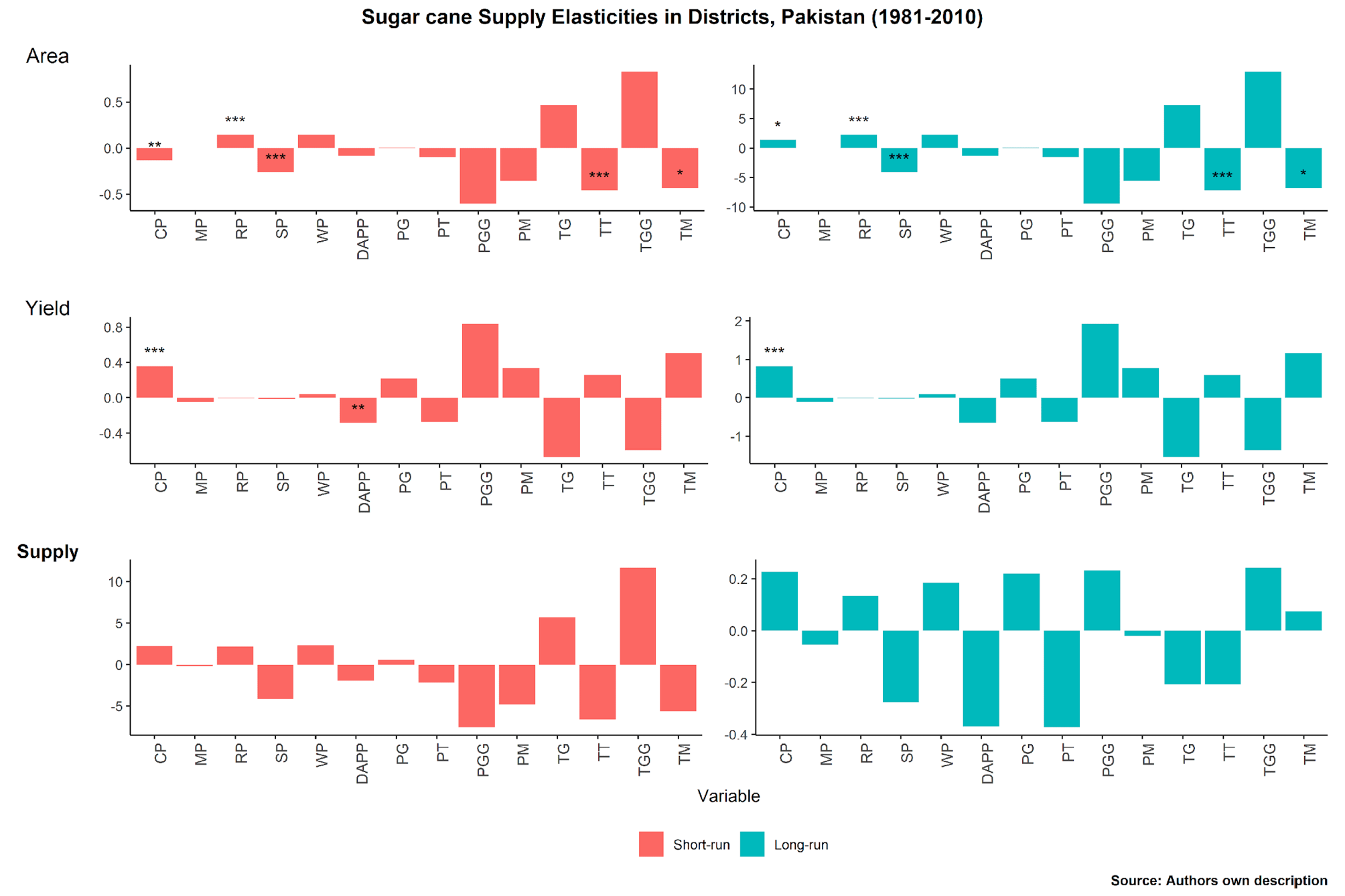
4.4. Elasticity of price and non-price factors
The rice and wheat prices have positive short-run elasticities, while the sugarcane price has a negative short-run elasticity for the area (Figure 3). Overall, the short-run price and non-price elasticities for the area response are very small, except for precipitation and temperature at the grand growth stage (β < 0.50). Regarding the yield response, four non-price factors – precipitation at grand growth (0.84%), temperature at germination (-0.67%), temperature at grand growth (-0.59%), and temperature at maturity (0.51%) – show higher short-run elasticities. Overall, price leads to positive changes in the sugarcane supply response: a 1% average price increase may increase the supply response by 0.07% in the long run. Non-price factors, such as precipitation and temperature, have negative long-run elasticities. This outcome confirms that the average non-price supply response is higher than price responses, and in the long run, acreage does not increase with the price (Siegle et al., 2024).
The sustainability of the sugarcane supply chain in Pakistan is at risk. The historic agriculture pricing policy has been inconsistent and ineffective and disincentivised [sugarcane] farmers to ensure the food system is resilient and sustainable. Sugarcane farmers behave idiosyncratically due to incoherent changes in agricultural policy and the inherent, invisible monopsony in the sugar[cane] market. Farmers have had to make trade-offs to find an optimal farm mix. Some of the paradoxical responses of growers may be explained by speculative behaviour driven by persistently higher [cane] sugar prices, leading to an expansion of the sugarcane area rather than an increase in yield.
Our study reveals that the previous sugarcane supply response findings require revalidation because important determinants have been excluded. In the long run, climate change undoubtedly influences the sugarcane supply response. However, these impacts are not uniform across the region or across all crops throughout the entire agricultural production cycle. Temperature has a more pronounced effect on the cropped area than on yield in the absence of sufficient R&D expenditure. These funds are crucial to mitigating the impact of climate change by developing new, area-specific, drought-tolerant, and/or heat-resistant varieties. Moreover, the volatility of input prices (i.e., DAP prices) has led to inefficient resource use and reduced sugarcane productivity.
The sustainability of the sugarcane supply chain depends on the introduction of radical, robust policy initiatives in the sugarcane market. These policy initiatives may be introduced as a sugarcane sector reform package. It should provide remedial measures to address the power imbalance between farmers and cane sugar manufacturers, promote competition, eradicate mill monopolistic abuse, and improve industry competitiveness. This can be achieved by removing unnecessary regulatory prerequisites and/or barriers to setting up and running new sugar mills (this issue requires further investigation), and by increasing R&D expenditure to modernise the sugarcane supply chain and ensure its resilience and responsiveness to real-world agricultural challenges.
The author (s) are sincerely thankful to Dr Munir Ahmad (Ex-Joint Director), Dr Muhammad Iqbal (Ex-Chief of Research) from the Pakistan Institute of Development Economics, Islamabad, and his team for providing the technical support, data, and guidance in completing this research. We thank Mr Muhammad Bilal Iqbal (Senior Scientific Officer), Climate Change, Alternate Energy & Water Resources Institute (CAEWRI), NARC, Islamabad, for his assistance in finalising Figure 1.> The principal author (ZM) worked as a research fellow at the International Development and Research Centre (IDRC), a Canada-funded project entitled Climate Change Adaptation, Water and Food Security in Pakistan.
Z.M.: Conceptualization, Data curation, Formal analysis, Investigation, Methodology, Writing—original draft preparation & review/editing.
G.V.: Methodology, Validation, Writing—review and editing, and Visualization.
M.C.: Supervise, Validate, and write—review and edit. All authors have read and agreed to the published version of the manuscript.
Abraham M., Pingali P. (2021). Shortage of pulses in India: understanding how markets incentivize supply response. Journal of Agribusiness in Developing and Emerging Economies, 11(4): 411-434. DOI: https://doi.org/10.1108/JADEE-11-2017-0128.
Abrar S., Morrissey O., Rayner T. (2004). Crop-level supply response by agro-climatic region in Ethiopia. Journal of Agricultural Economics, 55(2): 289-311. DOI: https://doi.org/10.1111/j.1477-9552.2004.tb00097.x.
Ali M. (1990). The price response of major crops in Pakistan: an application of the simultaneous equation model. The Pakistan Development Review, 29(3/4): 305-325.
Ali M., Ahmed F., Channa H., Davies S. (2016). Pakistan’s fertilizer sector: structure, policies, performance, and impacts. International Food Policy Research Institute (IFPRI), Washington, DC, USA.
Alston J.M., Chalfant J.A. (1991). Unstable models from incorrect forms. American Journal of Agricultural Economics, 73(4): 1171-1181. DOI: https://doi.org/10.2307/1242445.
Alston J.M., Sexton R.J., Zhang M. (1997). The effects of imperfect competition on the size and distribution of research benefits. American Journal of Agricultural Economics, 79(4): 1252-1265. DOI: https://doi.org/10.2307/1244282.
Antle J.M. (1983). Incorporating risk in production analysis. American Journal of Agricultural Economics, 65(5): 1099-1106. DOI: https://doi.org/10.2307/1240428.
Babcock B.A. (2015). Extensive and intensive agricultural supply response. Annual Review of Resource Economics, 7(1): 333-348. DOI: https://doi.org/10.1146/annurev-resource-100913-012424.
Bassu S., Brisson N., Durand J., Boote K., Lizaso J., Jones J.W., Rosenzweig C., Ruane A.C., Adam M., Baron C., Basso B., Biernath C., Boogaard H., Conijn S., Corbeels M., Deryng D., De Sanctis G., Gayler S., Grassini P., Hatfield J., Hoek S., Izaurralde C., Jongschaap R., Kemanian A.R., Kersebaum K.C., Kumar N.S., Makowski D., Müller C., Nendel C., Priesack E., Pravia M.V., Kim S., Sau F., Shcherbak I., Tao F., Teixeira E., Timlin D., Waha K. (2014). How do various maize crop models vary in their responses to climate change factors? Global Change Biology, 20(7): 2301-2320. DOI: https://doi.org/10.1111/gcb.12520.
Baum C.F., Schaffer M.E., Stillman S. (2003). Instrumental variables and GMM: estimation and testing. The Stata Journal, 3(1): 1-31. DOI: https://doi.org/10.1177/1536867X0300300101.
Boansi D. (2014). Yield response of rice in Nigeria: a co-integration analysis. American Journal of Agriculture and Forestry, 2(2): 15. DOI: https://doi.org/10.11648/j.ajaf.20140202.11.
Bor O., Bayaner A. (2009). How responsive is the crop yield to producer prices? A panel data approach for the case of Turkey. New Medit, 4.
Chavas J., Rivieccio G., Di Falco S., De Luca G., Capitanio F. (2022). Agricultural diversification, productivity, and food security across time and space. Agricultural Economics, 53(S1): 41-58. DOI: https://doi.org/10.1111/agec.12742.
Chavas J.-P., Di Falco S. (2017). Resilience, weather and dynamic adjustments in agroecosystems: the case of wheat yield in England. Environmental and Resource Economics, 67(2): 297-320. DOI: https://doi.org/10.1007/s10640-015-9987-9.
Chavas J.-P., Di Falco S., Adinolfi F., Capitanio F. (2019). Weather effects and their long-term impact on the distribution of agricultural yields: evidence from Italy. European Review of Agricultural Economics, 46(1): 29-51. DOI: https://doi.org/10.1093/erae/jby019.
Chen C.C., Chang C.C. (2005). The impact of weather on crop yield distribution in Taiwan: some new evidence from panel data models and implications for crop insurance. Agricultural Economics, 33(Supplement): 503-511. DOI: https://doi.org/10.1111/j.1574-0864.2005.00097.x.
Chen S., Yang J., Kang X. (2023). Effect of fiscal expenditure for supporting agriculture on agricultural economic efficiency in central China—a case study of Henan province. Agriculture, 13(4): 822. DOI: https://doi.org/10.3390/agriculture13040822.
de Medeiros Silva W.K., de Freitas G.P., Coelho Junior L.M., de Almeida Pinto P.A.L., Abrahão R. (2019). Effects of climate change on sugarcane production in the state of Paraíba (Brazil): a panel data approach (1990-2015). Climatic Change, 154(1-2): 195-209. DOI: https://doi.org/10.1007/s10584-019-02424-7.
Devadoss S., Luckstead J. (2010). An analysis of apple supply response. International Journal of Production Economics, 124(1): 265-271. DOI: https://doi.org/10.1016/j.ijpe.2009.11.024.
Đokić D., Novaković T., Tekić D., Matkovski B., Zekić S., Milić D. (2022). Technical efficiency of agriculture in the European Union and Western Balkans: SFA method. Agriculture, 12(12): 1992. DOI: https://doi.org/10.3390/agriculture12121992.
Doukas Y.E.L., Maravegias N., Chrysomallidis C. (2022). Digitalization in the EU agricultural sector: Seeking a European policy response. In Mattas K., Baourakis G., Zopounidis C., Staboulis C. (eds), Food Policy Modelling: Response to Current Issues (pp. 83-98). Springer, Cham. DOI: https://doi.org/10.1007/978-3-031-08317-4_6.
Ebrahim M.K., Zingsheim O., El-Shourbagy M.N., Moore P.H., Komor E. (1998). Growth and sugar storage in sugarcane grown at temperatures below and above optimum. Journal of Plant Physiology, 153(5-6): 593-602. DOI: https://doi.org/10.1016/S0176-1617(98)80209-5.
Edison E., Renate D., Denmar D. (2020). Dynamic supply response: implications for Indonesia soyabean crop. Dinasti International Journal of Economics, Finance Accounting, 1(4): 568-580. DOI: https://doi.org/10.38035/dijefa.v1i4.530.
Elnagheeb A.H., Florkowski W.J. (1993). Modeling perennial crop supply: An illustration from the pecan industry. Journal of Agricultural and Applied Economics, 25(1): 187-196. DOI: https://doi.org/10.1017/S1074070800018745.
FAO (2019). The State of the World’s Biodiversity for Food and Agriculture, FAO Commission on Genetic Resources for Food and Agriculture Assessments, Rome. http://www.fao.org/3/CA3129EN/CA3129EN.pdf.
Fligstein N., Calder R. (2015). Architecture of markets. In Scott R.A., Kosslyn S.M., Buchmann M. (eds) Emerging Trends in the Social and Behavioral Sciences (pp. 1-14). John Wiley Sons, Inc., Hoboken, NJ, USA. DOI: https://doi.org/10.1002/9781118900772.etrds0014.
Gliessman S. (2021). Transforming the food system: what does it mean? Agroecology and Sustainable Food Systems, 45(3): 317-319. DOI: https://doi.org/10.1080/21683565.2021.1842303.
Gohain N. (2018). An analysis of problems and constraints faced by farmers in marketing of agricultural produce in Punjab. Economic Affairs, 63(3). https://doi.org/10.30954/0424-2513.3.2018.11
Haile M.G., Kalkuhl M., Von Braun J. (2016). Worldwide acreage and yield response to international price change and volatility: a dynamic panel data analysis for wheat, rice, corn, and soybeans. American Journal of Agricultural Economics, 98(1): 172-190. DOI: https://doi.org/10.1093/ajae/aav013
Hannay J.W., Payne B.K. (2022). Effects of aggregation on implicit bias measurement. Journal of Experimental Social Psychology, 101, 104331. DOI: https://doi.org/10.1016/j.jesp.2022.104331
Hazrana J., Kishore A., Roy D. (2020). Supply response of staple food crops in the presence of policy distortions: some evidence from India. Agricultural Applied Economics Association Annual Meeting, Kansas City, MO, 1-25.
He L., Jin N., Yu Q. (2020). Impacts of climate change and crop management practices on soybean phenology changes in China. Science of the Total Environment, 707, 135638. DOI: https://doi.org/10.1016/j.scitotenv.2019.135638.
Hertel T.W. (2011). The global supply and demand for agricultural land in 2050: a perfect storm in the making? American Journal of Agricultural Economics, 93(2): 259-275. DOI: https://doi.org/10.1093/ajae/aaq189.
Hussain A., Khan A.A. (2021). Wild birds trade in Dera Ismael Khan and Bannu divisions of Khyber PakhtunKhwa (KPK) province, Pakistan. Brazilian Journal of Biology, 83. DOI: https://doi.org/10.1590/1519-6984.247915.
Jahangir M.H., Danehkar S. (2022). A comparative drought assessment in Gilan, Iran using Pálfai drought index, de Martonne aridity index, and Pinna combinative index. Arabian Journal of Geosciences, 15(1): 90. DOI: https://doi.org/10.1007/s12517-021-09107-7.
Kalaiselvi K., Sujarani P., Sakthivel V. (2024). Cropping pattern in farming. In Kalaiselvi K., Anand A.J., Tanwar P., Raza H. (eds) Advanced Technologies for Smart Agriculture (pp. 1-18). River Publishers, Gistrup.
Khan R., Hussain S.M.A. (2007). Farm supply response to price: a case study of sugarcane in Pakistan (1986 -2005). Journal of Independent Studies and Research, 5(2).
Khushk A.M., Memon A., Saeed I. (2011). Analysis of sugar industry competitiveness in Pakistan. Journal of Agriculture Research, 1(49).
Krishna R. (1963). Farm supply response in India-Pakistan: a case study of the Punjab region. The Economic Journal, 73(291): 477. DOI: https://doi.org/10.2307/2228581.
Lavanya B.T., Manjunatha A.V. (2025). Invisible monopsony in Indian sugar sector. Sugar Tech, 27(2): 318-327. DOI: https://doi.org/10.1007/s12355-024-01499-6.
Liu X., Lehtonen H., Purola T., Pavlova Y., Rötter R., Palosuo T. (2016). Dynamic economic modelling of crop rotations with farm management practices under future pest pressure. Agricultural Systems, 144: 65-76. DOI: https://doi.org/10.1016/j.agsy.2015.12.003.
Lobell D.B., Hammer G.L., McLean G., Messina C., Roberts M.J., Schlenker W. (2013). The critical role of extreme heat for maize production in the United States. Nature Climate Change, 3(5): 497-501. DOI: https://doi.org/10.1038/nclimate1832.
Lobell D.B., Roberts M.J., Schlenker W., Braun N., Little B.B., Rejesus R.M., Hammer G.L. (2014). Greater sensitivity to drought accompanies maize yield increase in the U.S. Midwest. Science, 344(6183): 516-519. DOI: https://doi.org/10.1126/science.1251423.
Mai C., Lin S. (2021). The effects of uncertainties over R&D policy or market demand on R&D levels. Managerial and Decision Economics, 42(4): 1048-1056. DOI: https://doi.org/10.1002/mde.3291.
Mbua I.A., Atta-Aidoo J. (2023). Acreage supply response of sugarcane out-growers in Tanzania: a vector error correction model (VECM) approach. Cogent Food Agriculture, 9(1). DOI: https://doi.org/10.1080/23311932.2023.2229575.
Mearns L.O., Rosenweig C., Goldberg R. (1997). Mean and variance change in climate scenarios: Methods, agricultural applications, and measures of uncertainty. Climate Change, 35: 367-396. DOI: https://doi.org/10.1023/A:1005358130291.
Mendelsohn B.R., Nordhaus W.D., Shaw D. (1994). The impact of global warming on agriculture: a Ricardian analysis. The American Economic Review, 84(4): 753-771. https://www.jstor.org/stable/2118029.
Mivumbi M., Yuan X. (2023). Sustainable environmental economics in farmers’ production factors via irrigation resources utilization using technical efficiency and allocative efficiency. Sustainability, 15(5), 4101. DOI: https://doi.org/10.3390/su15054101.
Mushtaq K., Dawson P.J. (2002). Acreage response in Pakistan: a co-integration approach. Agricultural Economics, 27: 111-121. DOI: https://doi.org/10.1016/S0169-5150(02)00031-2.
Mustafa G., Latif I.A. Egwuma, H. (2016). An empirical analysis of supply response of rubber in Malaysia. American Journal of Agricultural and Biological Sciences, 11(4): 148-156. DOI: https://doi.org/10.3844/ajabssp.2016.148.156.
Mustafa Z., Vitali G., Huffaker R., Canavari M. (2024). A systematic review on price volatility in agriculture. Journal of Economic Surveys, 38(1): 268-294. DOI: https://doi.org/10.1111/joes.12549.
Nelson G.C., Valin H., Sands R.D., Havlík P., Ahammad H., Deryng D., Elliott J., Fujimori S., Hasegawa T., Heyhoe E., Kyle P., von Lampe M., Lotze-Campen H., d’Croz D.M., van Meijl H., van der Mensbrugghe D., Müller C., Popp A., Robertson R., Robinson S., Schmid E., Schmitz C., Tabeau A., Willenbockel D. (2014). Climate change effects on agriculture: Economic responses to biophysical shocks. Proceedings of the National Academy of Sciences of the United States of America, 111(9): 3274-3279. DOI: https://doi.org/10.1073/pnas.1222465110.
Ngoc L.N.B., Thong L.Q., Hoa T.A. (2022). An analysis of supply response of black tiger shrimp production using Nerlove model: a case study of the Vietnamese Mekong delta. In Nguyen A.T., Hens L. (eds) Global Changes and Sustainable Development in Asian Emerging Market Economies (Vol. 1, pp. 121-131). Springer, Cham. DOI: https://doi.org/10.1007/978-3-030-81435-9_9
Nkang N.M., Ndifon H.M., Edet E.O. (2007). Maize supply response to changes in real prices in Nigeria: a vector error correction approach. Agricultural Journal, 2(3): 419-425.
Nosheen M., Iqbal J. (2008). Acreage response of major crops in Pakistan (1970-71 to 2006-07). ARPN Journal of Agricultural and Biological Science, 3(6): 55-64.
Osborne T. (2005). Imperfect competition in agricultural markets: evidence from Ethiopia. Journal of Development Economics, 76(2): 405-428. DOI: https://doi.org/10.1016/j.jdeveco.2004.02.002.
Pakistan Sugar Mills Association (2000). Annual Report 2000. Islamabad. Retrieved from https://www.psmacentre.com/documents/Annual%20Report%202000.pdf.
Pakistan Sugar Mills Association (2021). Annual Report 2021. Islamabad. Retrieved from https://www.psmacentre.com/documents/PSMA%20Annual%20Report%20Final%20%202021.pdf.
Pardey P.G., Beintema N.M., Dehmer S., Wood S. (2006). Agricultural research: A growing global divide? Food Policy Report No. 17. International Food Policy Research Institute.
Pirzada A.J., Shahid N., Ghauri R.T. (2023). The ongoing crisis in the sugar industry: The implications of legislations and need of deregulation. The Pakistan Development Review, 62(4): 553-572. DOI: https://doi.org/10.30541/v62i4pp.553-572.
Ray D.K., Ramankutty N., Mueller N.D., West P.C., Foley J.A. (2012). Recent patterns of crop yield growth and stagnation. Nature Communications, 3(1): 1293. DOI: https://doi.org/10.1038/ncomms2296.
Rezaei E.E., Siebert S., Hüging H., Ewer, F. (2018). Climate change effect on wheat phenology depends on cultivar change. Scientific Reports, 8(1): 4891. DOI: https://doi.org/10.1038/s41598-018-23101-2.
Saddiq M., Fayaz M., Hussain Z., Shahab M., Ullah I. (2013). Acreage response of sugarcane to price and non price factors in Khyber Pakhtunkhwa. International Journal of Food and Agricultural Economics, 2(3): 121-128. DOI: https://10.22004/ag.econ.186272.
Santeramo F.G., Miljkovic D., Lamonaca E. (2021). Agri-food trade and climate change. Economia Agro-Alimentare, 1: 1-18. DOI: https://doi.org/10.3280/ecag1-2021oa11676.
Shafique M., Hussain Z., Sial M. (2007). Supply response function of sugarcane crop in Punjab, Pakistan. European Journal of Scientific Research, 17(2): 277-290.
Shehzad M., Zahid N., Maqbool M., Singh A., Liu H., Wu C., Khan A., Wahid F., Saud S. (2022). Climate resilience in agriculture. In Jatoi W.N., Mubeen M., Ahmad A., Cheema M.A., Lin Z., Hashmi M.Z. (eds) Building Climate Resilience in Agriculture: Theory, Practice and Future Perspective (pp. 67-82). Springer, Cham. DOI: https://doi.org/10.1007/978-3-030-79408-8_5.
Siegle J., Astill G., Plakias Z., Tregeagle D. (2024). Estimating perennial crop supply response: a methodology literature review. Agricultural Economics, 55(2): 159-180. DOI: https://doi.org/10.1111/agec.12812.
Skogstad G. (1993). Policy under siege: supply management in agricultural marketing. Canadian Public Administration, 36(1): 1-23.
Tao F., Yokozawa M., Xu Y., Hayashi Y., Zhang Z. (2006). Climate changes and trends in phenology and yields of field crops in China, 1981-2000. Agricultural and Forest Meteorology, 138(1-4): 82-92. DOI: https://doi.org/10.1016/j.agrformet.2006.03.014.
Tenaye A. (2020). New evidence using a dynamic panel data approach: cereal supply response in smallholder agriculture in Ethiopia. Economies, 8(3): 61. DOI: https://doi.org/10.3390/economies8030061.
Thornton P.K., Ericksen P.J., Herrero M., Challinor A.J. (2014). Climate variability and vulnerability to climate change: a review. Global Change Biology, 20(11): 3313-3328. DOI: https://doi.org/10.1111/gcb.12581.
U.S. Department of Agriculture, Foreign Agricultural Service. (2021, April 22). Sugar annual: Pakistan. Islamabad. Report No. PK2021-0006 [GAIN Report]. https://apps.fas.usda.gov/newgainapi/api/Report/DownloadReportByFileName?fileName=Sugar%20Annual_Islamabad_Pakistan_04-15-2021.pdf.
Van Der Wiel K., Bintanja R. (2021). Contribution of climatic changes in mean and variability to monthly temperature and precipitation extremes. Communications Earth Environment, 2(1): 1. DOI: https://doi.org/10.1038/s43247-020-00077-4.
Vasantha S., Shekinah D.E., Gupta C., Rakkiyappan P. (2012). Tiller production, regulation and senescence in sugarcane (saccharum species hybrid) genotypes. Sugar Tech, 14(2): 156-160. DOI: https://doi.org/10.1007/s12355-011-0129-6.
Verma R.R., Srivastava T.K., Singh P. (2019). Climate change impacts on rainfall and temperature in sugarcane growing Upper Gangetic Plains of India. Theoretical and Applied Climatology, 135(1-2): 279-292. DOI: https://doi.org/10.1007/s00704-018-2378-8.
Von Cramon-Taubadel S., Goodwin B.K. (2021). Price transmission in agricultural markets. Annual Review of Resource Economics, 13(1): 65-84. DOI: https://doi.org/10.1146/annurev-resource-100518-093938.
Wang Y., Wang J., Wang X. (2020). COVID-19, supply chain disruption and China’s hog market: A dynamic analysis. China Agricultural Economic Review, 12(3): 427-443. DOI: https://doi.org/10.1108/CAER-04-2020-0053.
Wani M.H., Sehar H., Paul R.K., Kuruvila A., Hussain I. (2015). Supply response of horticultural crops: The case of apple and pear in Jammu & Kashmir. Agricultural Economics Research Review, 28(1): 83. DOI: https://doi.org/10.5958/0974-0279.2015.00006.3.
Wasim M.P. (1997). Sugarcane acreage response in Sindh - Pakistan. Pakistan Journal of Applied Economics, 2(1): 143-156.
Wu J., Adams R.M. (2002). Micro versus macro acreage response models: does site-specific information matter? Journal of Agricultural and Resource Economics, 27(1): 40-60. DOI: https://doi.org/10.22004/ag.econ.31074.
Yaseen M.R., Dronne Y. (2011). Estimating the supply response of main crops in developing countries: the case of Pakistan and India. ARPN Journal of Agricultural and Biological Science, 6(10): 78-87.
Yu B., Liu F., You L. (2012). Dynamic agricultural supply response under economic transformation: a case study of Henan, China. American Journal of Agricultural Economics, 94(2): 370-376. DOI: https://doi.org/10.1093/ajae/aar114.
Yu C., Miao R., Khanna M. (2021). Maladaptation of U.S. corn and soybeans to a changing climate. Scientific Reports, 11(1), 12351. DOI: https://doi.org/10.1038/s41598-021-91192-5.
Yu J., Smith A., Sumner D.A. (2018). Effects of crop insurance premium subsidies on crop acreage. American Journal of Agricultural Economics, 100(1): 91-114. DOI: https://doi.org/10.1093/ajae/aax058.